This blog post was originally published at Qualcomm’s website. It is reprinted here with the permission of Qualcomm.
Before I joined Qualcomm Technologies Netherlands, computation was always a black box for me. I’d design an algorithm, code it up in some high-level programming language, run it, and it would simply work. Since then, I have learnt that computation is a marvel of technology, from the design and fabrication of the chip, to the mapping of the computation onto the hardware, to the actual computation in terms of bits.
I have also learnt that one of the constraining factors of computation is its power consumption. This is true for economic reasons: if the economic return obtained by performing some computation is less than the energy bill, it makes no financial sense to perform it. Also, energy needs to be dissipated, otherwise a phone in your pocket can get hot and will need to run at lower performance. Given this, I predict that increasingly we will measure success in the field of AI by the amount of intelligence we can generate per joule. Not coincidentally, this is also true for biological intelligence because for every joule burnt in your brain you need to find food to pay for the energy bill. And let’s be clear, there is still a lot of room for improvement here: the human brain, which has evolved over millions of years, is estimated by some to be around 100,000 times more energy efficient than our best silicon hardware.
And so, at Qualcomm AI Research we think about how to design energy-efficient machine learning that runs well on our hardware, and at the same time influence the hardware designers to build better specialized (ASIC) chips to run machine learning workloads. In essence, we are co-designing the hardware, software, and algorithms. There are multiple ways to approach this, such as trimming down the neural network, optimizing the compilation of the computation onto hardware (for instance, by avoiding the movement of data back and forth between off-chip and on-chip memory), or reducing the precision of computation by reducing the number of available bits (a.k.a. quantization). I was especially intrigued by the latter: how can you adaptively determine the required precision for a prediction task?
This question is particularly interesting in a neural network where adding noise to the hidden layers seems to actually improve its generalization performance. Adding high-precision noise to high-precision random variables seems silly. We asked ourselves the question: can we learn from the data how many bits a certain computation kernel needs? The information stored in the data should be transferred to the variables of the model, so a large dataset should translate to high-precision parameters while a small dataset should translate to noisy, low-precision parameters. In the extreme case the model might even decide to use zero bits for some parameter which would be equivalent to pruning the parameter away.
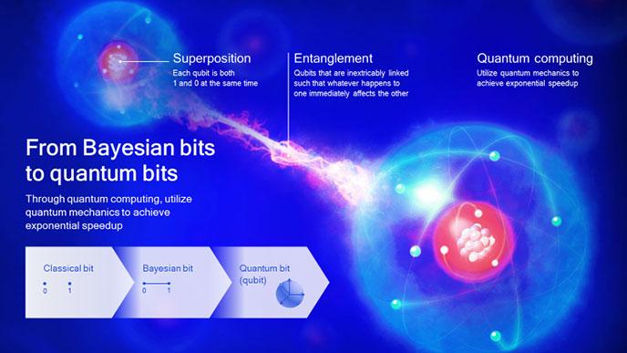
Bayesian bits
This problem can be approached by using Bayesian statistics. In Bayesian statistics we maintain a probability distribution for every variable, and since a variable can be expressed in terms of a bit string, this translates to a probability for each bit. We can call this a “Bayesian bit.” A Bayesian probability is a subjective probability of your belief about the state of the world. It is a property of your brain and not of the world. Each one of us will entertain different beliefs about the world because we are all privy to different observations. And hopefully we will update these subjective probabilities in light of new evidence1.
Our Bayesian bits method works a bit like a sequence of gates. Given our dataset, we first determine if there is enough evidence to include a parameter in the computation. Given that we decided it is a useful parameter we continue to determine if we need a second bit to represent it. This process continues until a gate closes, implying that all less significant bits will be removed. Through this idea we were able to adaptively determine the necessary precision for a computation and save energy in the process.
Quantum bits
By probabilistically reasoning about individual bits it seems that we have reached the most fundamental level of information processing and computation. “Can we still go a level deeper?”, was the next natural question to ask. And amazingly, the answer is yes, because nature actually doesn’t use probabilistic bits, but rather quantum bits (or “qubits”). To understand the difference, and the implications of the difference, let’s first formalize probabilistic bits a bit more.
A classical bit can take two values x=(0,1). A probabilistic bit however can take values p(x)=(q,1-q), where q is any real number between 0 and 1 representing the probability of taking on value 0. Probabilistic bits can be “entangled,” which is just to say that their values can be correlated. For two bits we have four possible states x=(00,01,10,11). For entangled bits the probabilities for x are dependent, that is, if we know the value for one x, then we also know something about the value for another x. In the notation above, a vector p(x)=(½,0,0,½) would represent an entangled bit pair. As an example, consider the colour values of two neighbouring pixels in an image. Given one pixel value, you can predict with high probability the value of the other, and so their values are entangled.
Probabilities also have the convenient property that they add up. If there are two paths from A to C, one through B1 and the other through B2, then the probability of getting to C is the sum of the probabilities of the two paths through B1 and B2.

Classical probability theory where the sum of all probabilities equals one.
To understand qubits2 we need to make a seemingly inconsequential change to the definition of how to represent information. Instead of using positive numbers, p, that sum to one we will now use complex numbers whose (absolute) squares sum to one. We call these probability amplitudes. For the sake of the argument, you can forget the complex number part and just replace p with plus or minus the square root of p. For the case of one qubit we would thus have two numbers a and b that lie on a circle: a2 + b2 = 1. This looks remarkably similar to the case of probabilistic bits, but as we will see, it will have large consequences.

Qubits have the properties of superposition and entanglement, which can enable exponential speedup in computing.
Just like probabilistic bits, qubits can also be entangled, which also roughly means that their values are dependent. In math notation, a (maximally) entangled pair of qubits is represented by the probability amplitude ψ(x)=(1/√2,0,0,1/√2). A famous thought experiment, that was later validated in the lab, is the so-called Einstein-Podolsky-Rosen paradox, first conjured up by Einstein and colleagues to show that quantum mechanics could not possibly be correct. Two friends each get one of two maximally entangled qubits and they take them to the other sides of the galaxy. If the first friend performs an experiment, and reads out the value, then the outcome of the experiment of the second friend on the other side of the galaxy is now fully determined, instantaneously.
When you read this, you get a strong feeling that these probability amplitudes must also describe our subjective knowledge about the world. How else could this information “travel” faster than the speed of light? And while this issue is still hotly debated3, most physicists today believe that wavefunctions indeed represent the actual state of the world, and not the state of our brain.
Besides these strange “action at a distance” effects, there is a more immediate consequence of using amplitudes, namely that they can cancel each other out, which is called interference. To understand this let’s again consider two paths going from A to C, one through B1 and one through B2. In the classical case, the paths had positive weights which were added together. But in the quantum world we need to add the probability amplitudes before we take the squares to compute probabilities. So, let’s assume the amplitude of a particle at C going through B1 is a, and the amplitude going through B2 is -a, then their sum is 0, and you will find that there is no particle at C. This is particularly strange because you can measure particles at B1 and B2 but just like waves they can destructively interfere at C. If the particle is on its way on one of the two paths it must be somehow aware of the other path (and in general all possible paths), implying that it is everywhere at the same time!

Quantum probabilities exhibit interesting properties, such as being everywhere at the same time.
Now, this property of a quantum amplitude to be everywhere at once, can be translated for qubits to be in all possible states at once. So, one qubit is in two states at once, two qubits in four states at once, three qubits in eight states at once and 100 qubits in 1,300000000000000000000000000000 states at once. Quantum computers can simultaneously manipulate these amplitudes over exponentially many states. And it is this property that makes quantum computers potentially so powerful4 (read our paper, Quantum Deformed Neural Networks).
There are currently three successful approaches to quantum computing: two based on qubits (superconducting qubits and trapped ions) and one based on photonics (i.e., light). The optical quantum computers operate with so called continuous variable states as opposed to the discrete qubits. One may model an image as a two-dimensional (quantum) field of oscillators where the amplitude of the oscillator at pixel i corresponds to pixel values of the image. Neighbouring pixels will be entangled (correlated) and thus one can picture waves propagating through this grid like ripples in a pond of water.
A quantum computation is a sequence of operations on this quantum field decomposed in elementary gates. We have linear operators implemented by beam-splitters, phase shifters, and squeezers, and amazingly these can be mapped onto the linear layers of a neural network. And, just as with neural networks, there are also nonlinear operators in a quantum circuit. Inspired by the ReLU we invented a new nonlinear gate that implements a soft version of the ReLU in an optical quantum circuit.
All in all, the similarities between an optical quantum circuit in the continuous variable representation and a neural network are uncanny. This means that we can probably quite easily implement a neural network on an optical quantum computer. But whether this will result in more powerful machine learning models is highly speculative and remains a wide-open research question.
The Hinton
One particularly amusing aspect of formulating a neural network in the language of quantum field theory is that we can identify elementary particles as the fundamental excitations of these quantum fields (quantized ripples in the pond). We thought that the name “hinton” was fitting for the first neural particle ever discovered5 (read our paper, The Hintons in your Neural Network: a Quantum Field Theory View of Deep Learning). The computation that is happening inside the guts of a neural network can thus be understood as gazillions of hintons interacting together to orchestrate a prediction.

We’ve named the first neural particle ever discovered to be, the hinton.
We hope that our work will inspire many others to continue on this exciting path of quantum machine learning.
1In today’s society with misinformation all around us, this is increasingly challenging.
2Feynman seemed to have said: “if you think you understand quantum mechanics you don’t understand quantum mechanics.”
3The author still believes that probabilistic amplitudes do indeed describe subjective quantities.
4Quantum computers are very fast for a restricted set of computations, not all computations.
5Named after Geoffrey Hinton, the founding father of deep learning.
Dr. Max Welling
Vice President, Technology, Qualcomm Technologies