
By Michael Tusch
Founder and CEO
Apical Limited
Camera designers have decades of experience in creating image processing pipelines which produce attractive and/or visually accurate images, but what kind of image processing produces video which is well-purposed for subsequent analytics? It seems reasonable to begin by considering a conventional ISP (image signal processor). After all, the human eye-brain system produces what we consider aesthetically pleasing imagery for a purpose: to maximize our decision-making abilities. But which elements of such an ISP are most important to get right for good analytics, and how do they impact the performance of the algorithms which run on them?
In this introductory article, we’ll survey the main components of an ISP, highlight those components whose performance we believe to be particularly important for good analytics, and discuss what their effect is likely to be. In subsequent articles, we'll look at specific algorithm co-optimizations between analytics and these main components, focusing on applications in object tracking and face recognition.
Figure 1 shows a simplified block schematic of a conventional ISP. The input is sensor data in a raw format (one color per pixel), and the output is interpolated RGB or YCbCr data (three colors per pixel).
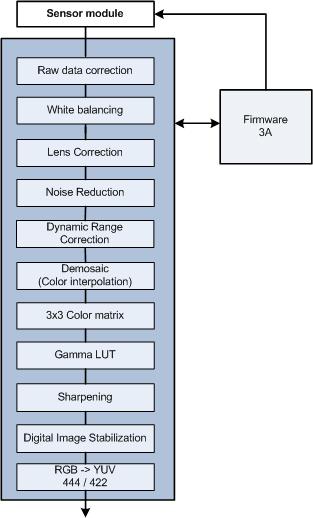
Figure 1. This block diagram provides a simplified view inside a conventional ISP (image signal processor)
Table 1 briefly summarizes the function of each block. The list is not intended to be exhaustive: an ISP design team will frequently also implement other modules.
| Module | Function |
| Raw data correction | Set black point, remove defective pixels. |
| Lens correction | Correct for geometric and luminance/color distortions. |
| Noise reduction | Apply temporal and/or spatial averaging to increase SNR (signal to noise ratio). |
| Dynamic range compression | Reduce dynamic range from sensor to standard output without loss of information. |
| Demosaic | Reconstruct three colors per pixel via interpolation with pixel neighbors. |
| 3A | Calculate correct exposure, white balance and focal position. |
| Color correction | Obtain correct colors in different lighting conditions. |
| Gamma | Encode video for standard output. |
| Sharpen | Edge enhancement. |
| Digital image stabilization | Remove global motion due to camera shake/vibration. |
| Color space conversion | RGB to YCbCr. |
Table 1. Functions of main ISP modules
Analytics algorithms may operate directly on the raw data, on the output data, or on data which has subsequently passed through a video compression codec. The data at these three stages often has very different characteristics and quality, which are relevant to the performance of analytics algorithms.
Let us now review the stages of the ISP in order of decreasing importance to analytics, which happens also to be approximately the top-to-bottom order shown in Figure 1. We start with the sensor and optical system. Obviously, the better the sensor and optics, the better the quality of data on which to base decisions. But "better" is not a matter simply of resolution, frame rate or SNR (signal-to-noise ratio). Dynamic range is also a key characteristic. Dynamic range is essentially the relative difference in brightness between the brightest and darkest details that the sensor can record within a single scene, normally expressed in dB.
Common CMOS and CCD sensors have a dynamic range of between 60 and 70 dB, which is sufficient to capture all details in scenes which are fairly uniformly illuminated. Special sensors are required, on the other hand, to capture the full range of illumination in high contrast environments. Around 90dB of dynamic range is needed to simultaneously record information in deep shadows and bright highlights on a sunny day; this requirement rises further if extreme lighting conditions occur (the human eye has a dynamic range of around 120dB). If the sensor can’t capture such a range, objects which move across the scene will disappear into blown-out highlights, or into deep shadows below the sensor black level. High (e.g. wide) dynamic range sensors are certainly helpful in improving analytics in uncontrolled lighting environments. Efficient processing of such sensor data is not trivial, however, as discussed below.
The next most important element is noise reduction, which is important for a number of reasons. In low light, noise reduction is frequently necessary to raise objects above the noise background, subsequently aiding in accurate segmentation. Also, high levels of temporal noise can easily confuse tracking algorithms based on pixel motion even though such noise is largely uncorrelated, both spatially and temporally. If the video go through a lossy compression algorithm prior to analytics post-processing, you should also consider the effect of noise reduction on compression efficiency. The bandwidth required to compress noisy sources is much higher than with "clean" sources. If transmission or storage is bandwidth-limited, the presence of noise reduces the overall compression quality and may lead to increased amplitude of quantization blocks, which easily confuses analytics algorithms.
Effective noise reduction can readily increase compression efficiency by 70% or more in moderate noise environments, even when the increase in SNR is visually not very noticeable. However, noise reduction algorithms may themselves introduce artifacts. Temporal processing works well because it increases the SNR by averaging the processing over multiple frames. Both global and local motion compensation may be necessary to eliminate false motion trails in environments with fast movement. Spatial noise reduction aims to blur noise while retaining texture and edges and risks suppressing important details. You must therefore strike a careful balance between SNR increase and image quality degradation.
The correction of lens geometric distortions, chromatic aberrations and lens shading (vignetting) is of inconsistent significance, depending on the optics and application. For conventional cameras, uncorrected data may be perfectly suitable for post-processing. In digital PTZ (point, tilt and zoom) cameras, on the other hand, correction is a fundamental component of the system. A set of "3A" algorithms control camera exposure, color and focus, based on statistical analysis of the sensor data. Their function and impact on analytics is shown in Table 2 below.
| Algorithm | Function | Impact |
| Auto exposure | Adjust exposure to maximize the amount of scene captured. Avoid flicker in artificial lighting. | A poor algorithm may blow out highlights or clip dark areas, losing information. Temporal instabilities may confuse motion-based analytics. |
| Auto white balance | Obtain correct colors in all lighting conditions. | If color information is used by analytics, it needs to be accurate. It is challenging to achieve accurate colors in all lighting conditions. |
| Auto focus | Focus the camera. | Which regions of the image should receive focus attention? How should the algorithm balance temporal stability versus rapid refocusing in a scene change? |
Table 2. The impact of "3A" algorithms
Finally, we turn to DRC (dynamic range compression). DRC is a method of non-linear image adjustment which reduces dynamic range, i.e. global contrast. It has two primary functions: detail preservation and luminance normalization.
I mentioned above that the better the dynamic range of the sensor and optics, the more data will typically be available for analytics to work on. But in what form do the algorithms receive this data? For soome embedded vision applications, it may be no problem to work directly with the high bit depth raw sensor data. But if the analytics is run in-camera on RGB or YCbCr data, or as post-processing based on already lossy-compressed data,the dynamic range of such data is typically limited by the 8-bit standard format, which corresponds to 60 dB. This means that, unless dynamic range compression occurs in some way prior to encoding, the additional scene information will be lost. While techniques for DRC are well established (gamma correction is one form, for example), many of these techniques decrease image quality in the process, by degrading local contrast and color information, or by introducing spatial artifacts.
Another application of DRC is in image normalization. Advanced analytics algorithms, such as those employed in facial recognition, are susceptible to changing and non-uniform lighting environments. For example, an algorithm may recognize the same face differently depending on whether the face is uniformly illuminated or lit by a point source to one side, in the latter case casting a shadow on the other side. Good DRC processing can be effective in normalizing imagery from highly variable illumination conditions to simulated constant, uniform lighting, as shown in Figure 2.
 |
 |
Figure 2. DRC (Dynamic range control) can normalize a source image with non-uniform illumination
In general, we find that the requirements of an ISP to produce natural, visually-accurate imagery and to produce well-purposed imagery for analytics are closely matched. However, as is well-known, it is challenging to maintain accuracy in uncontrolled environments. In future articles, we will focus on individual blocks of the ISP and consider the effect of their specific performance on the behavior of example analytics algorithms.