
By Michael Tusch
Founder and CEO
Apical Limited
This article will expand on the theme initiated in the premier article of this series, that of exploring how the pixel processing performed in cameras can either enhance or hinder the performance of embedded vision algorithms. Achieving natural or otherwise aesthetically pleasing camera images is normally considered distinct from the various tasks encompassed in embedded vision. But the human visual system has likely evolved to produce the images we perceive not for beauty per se, rather in order to optimize the brain's decision-making processes based on these inputs.
It may well be, therefore, that we in the embedded vision industry can learn something by considering the image creation and image analysis tasks in combination. While current architectures consider these tasks as sequential and largely independent stages, we also know that the human eye-brain system exhibits a high degree of feedback whereby the brain’s model of the environment informs the image capture process. In Apical's opinion, it is inevitable that future machine vision systems will be designed along similar principles.
In case all this sounds rather high-minded and vague, let’s focus on a specific example of how an imaging algorithm interacts with a simple vision algorithm, a case study that has immediate and practical consequences for those designing embedded vision systems. We’ll look at how the method of DRC (dynamic range compression), a key processing stage in all cameras, affects the performance of a simple threshold-based edge detection algorithm. This technique also happens to have a clear parallel in human vision, since both processes are performed with almost unparalleled efficiency within the eye, based on surprisingly simple and analog neural architectures.
DRC, also known as tone mapping, is the process by which an image with high dynamic range is mapped into an image with lower dynamic range. The term “dynamic range” refers to the relative intensity of the brightest details (as compared to the intensity of the darkest details) which can be resolved within a single image. Most real-world situations exhibit scenes with a dynamic range of up to ~100 dB, although there are conditions where the dynamic range is much higher, and the eye can resolve around 150 dB. Sensors exist which can capture this range or more, which equates to around 17-18 bits per color per pixel. Standard sensors capture around 70 dB, which corresponds to around 12 bits per color per pixel.
We would like to use as much information about the scene as possible for embedded vision, implying that we should use as many bits as possible as input data. One possibility is just to take this raw sensor data as-is, in linear form. But often this data is not available, as the camera module may be separate from the computer vision processor, with transmission subsequently limited to 8 bits per color per pixel. Also, some kinds of vision algorithms work better if they are presented with a narrower image dynamic range: less variation in the scene illumination consequently needs to be taken into account.
Often, therefore, some kind of DRC will be performed between the raw sensor data (which may in some cases be very high dynamic range) and the standard RGB or YUV output provided by the camera module. This DRC will necessarily be non-linear; the most familiar example is gamma correction. In fact, gamma correction is more correctly described as dynamic range preservation, because the intention is to match the gamma applied in-camera with an inverse function applied at the display, in order to recover a linear image at the output (as in, for example, the sRGB or rec709 standards for mapping 10-bit linear data into 8-bit transmission formats).
However, the same kind of correction can be and is also frequently used to compress dynamic range. For the purposes of our vision algorithm example, it would be best to work in a linear domain. In principle, it would be straightforward to apply an inverse gamma and recover the linear image as input. But unfortunately, the gamma used in the camera does not always follow a known standard. There’s a good reason for this: the higher the dynamic range of the sensor, the larger the amount of non-linear correction that needs to be applied to those images which actually exhibit high dynamic range. Conversely, for images that don’t fit the criteria, i.e. images of scenes that are fairly uniform in illumination, little or no correction should be applied.
As a result, the non-linear correction needs to be adaptive, meaning that the algorithm's function depends on the image itself, as derived from an analysis of the intensity histogram of the component pixels. And it may need also to be spatially varying, meaning that different transforms are applied in different image regions. The overall intent is to try to preserve as much information as accurately as possible, without clipping or distortion of the content, while mapping the high input dynamic range down to the relatively low output dynamic range. Figure 1 gives an example of what DRC can achieve: the left-hand image retains the contrast of the original linear sensor image, while the right-hand post-DRC image appears much closer to what the eye would observe.
 |
 |
Figure 1: Original linear image (left) and image after dynamic range compression (right)
Let us assume that we need to work with this non-linear image data as input to our vision algorithm, which is the normal case in many real-world applications. How will our edge detection algorithm perform on this type of data, as compared to the original linear data? Let us consider a very simple edge detection algorithm, based on the ratio of intensities of neighbouring pixels, such that an edge is detected if the ratio is above a pre-defined threshold. And let us also consider the simplest form of DRC, which is gamma-like, and might be associated with a fixed exponent or one derived from histogram analysis (i.e. “adaptive gamma”). What effect will this gamma function have on the edge intensity ratios?
The gamma function is shown in Figure 2, at top right. Here, the horizontal axis is the pixel intensity in the original image, while the vertical axis is the pixel intensity after gamma correction. This function increases the intensity of pixels in a variable manner, such that darker pixels have their intensities increased more than brighter pixels. Figure 2 (top left) shows an edge, with its pixel intensity profile along the adjacent horizontal line. This image is linear; it has been obtained from the original raw data without any non-linear intensity correction. Clearly, the edge corresponds to a dip in the intensity profile; let us assume that this dip exceeds our edge detection threshold by a small amount.
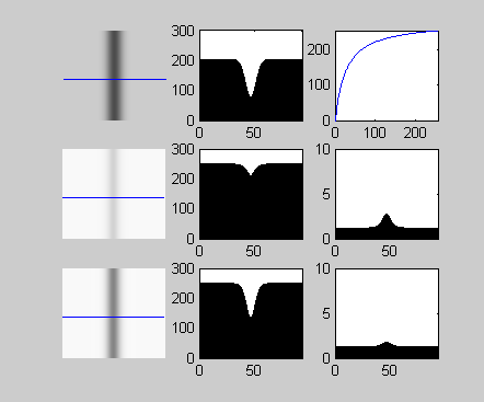
Figure 2: Effect of DRC on an edge. The original edge is shown in the top-left corner, with the gamma-corrected result immediately below it. The intensity profile along the blue horizontal line is shown in the middle column. The result of gamma correction is shown in the middle row, with the subsequent outcome of applied local contrast preservation correction shown in the bottom row.
Now consider the same image after the gamma correction (top right), as shown in Figure 2, middle row. The intensity profile has been smoothed out, with the amplitude of the dip greatly reduced. The image itself is brighter, but the contrast ratio is lower. The reason should be obvious: the pixels at the bottom of the dip are darker than the rest, and their intensities are therefore relatively increased more by the gamma curve than the rest, thereby closing the gap. The difference between the original and new edge profiles is shown in the right column. The dip is now well below our original edge detection threshold.
This outcome is problematic for edge detection, since the strengths of the edges present in the original raw image are reduced in the corrected image, moreover reduced in a totally unpredictable way based on where the edge occurs in the intensity distribution. Making the transform image-adaptive and spatially-variant further increases the unpredictability of how much edges will be smeared out by the transform. There is simply no way to relate the strength of edges in the output to those in the original linear sensor data. On the one hand, therefore, DRC is necessary to pack information recorded by the sensor into a form that the camera can output. However, this very process degrades important local pixel information needed for reliable edge detection.
The degradation could manifest as instability in the white line detection algorithm for an automotive vision system, particularly (for example) when entering or exiting a tunnel, where the dynamic range of the scene changes rapidly and dramatically. Fortunately, a remedy exists. The fix arises from an observation that an ideal DRC algorithm should be highly non-linear on large length scales on the order of the image dimensions, but should be strictly linear on very short scales of a few pixels. In fact this outcome is also desirable for other reasons. Let us see how it can be accomplished, and what effect it would have on the edge problem.
The technique involves deriving a pixel-dependent image gain via the formula Aij = Oij/D(Iij), where i,j are the pixel coordinates, O denotes the output image and I the input image, and D is a filter applied to the input image which acts to increase the width of edges. The so-called amplification map, A, is post-processed by a blurring filter which alters the gain for a particular pixel based on an average over its nearest neighbours. This modified gain map is multiplied with the original image to produce the new output image. The result is that the ratio in intensities between neighbouring pixels is precisely preserved, independent of the overall shape of the non-linear transform applied to the whole image.
This result is shown in the bottom row of Figure 2. Although the line is brighter, its contrast with respect to its neighbours is preserved. We can see this more clearly in the image portion example of Figure 3. Here, several edges are present within the text. The result of standard gamma correction is to reduce local contrast, “flattening” the image, while the effect of the local contrast preservation algorithm is to lock the ratio of edge intensities, such that the dips in the intensity profile representing the dark lines within the two letters in the bottom image and the top image are identical.
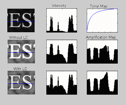
Figure 3: Effect of DRC on a portion of an image. The original linear image is in the top-left corner, with the gamma-corrected result immediately below it. The effect of local contrast preservation is shown in the bottom-left corner.
In summary, while non-linear image contrast correction is essential for forming images that are viewable and transmissible, such transforms should retain linearity on small scales important for edge analysis. Note that our definition of the amplification map above as a pixel position-dependent quantity implies that such transforms must be local rather than global (i.e. position-independent). It is worth noting that the vast majority of cameras in the market entirely employ global processing and therefore have no means of controlling the relationship between edges in the original linear sensor data and the camera output.
In conclusion, we have reviewed an example of where the nature of the image processing applied in-camera has a significant effect on the performance of a basic embedded vision algorithm. The data represented by a standard camera output is very different from the raw data recorded by the camera sensor. While in-camera processing is crucial in delivering images which accurately reflect the original scene, it may have an unintended negative impact on the effectiveness of vision algorithms. Therefore, it is a good idea to understand how the pixels input to the algorithms have been pre-processed, since this pre-processing may have both positive and negative impacts on the performance of those algorithms in real-life situations.
We will look at other examples of this interaction in future articles.