This article was originally published on June 10, 2015 at Altera's website. It is reprinted here with the permission of Altera.
Papers at this year’s Embedded Vision Summit suggested the vast range of ways that embedded systems can employ focused light as an input, and the even vaster range of algorithms and hardware implementations they require to render that input useful. Applications range from simple, static machine vision to classification and interpretation of real-time, multi-camera video. And hardware can range from microcontrollers to purpose-built supercomputers and arrays of neural-network emulators.
Perhaps surprisingly, most of the systems across this wide spectrum of requirements and implementations can be described as segments of a single processing pipeline. The simplest systems implement only the earliest stages of the pipeline. More demanding systems implement deeper stages, until we reach the point of machine intelligence, where all the stages of the pipeline are present, and may be coded into one giant neural-network model.
The individual stages are easy to describe, if not easy to implement (Figure 1). In the first stage, a—usually–simple algorithm extracts features from the image. Features, in this context, are easily-detectable patterns, such as edges, corners, or wavelets, that tend to be stable attribute of the object on which they occur, even when externalities like position or lighting change. The line- and arc-segments in printed characters or the patterns of light and dark regions in a human face are examples. Depending on what kind of features you are trying to extract, the best tool may be, for example, a convolution kernel scanning across the image, or a gradient-based matrix analysis looking for points at which the color or intensity of pixels changes dramatically.
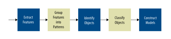
Figure 1. Most vision systems follow a predictable pipeline.
In the next stage, the system looks for patterns in the list of features. A simple system might look just for spatial relationships—is there a loop near the top of that vertical bar? Or the system might look for temporal relationships—how has each feature moved between this frame and the previous one: are there features that always move together? This search for patterns can be repeated to search for patterns among the patterns, and so on. These searches for patterns can be done by rule-based algorithms, or they can be done by convolutional networks.
The next stage is more challenging: locating objects. In the abstract sense, an object is a persistent set of patterns that appear to be grouped together by some associating factor, such as being next to each other, being all the same color, being surrounded by a boundary of edges, or all moving together, to cite some examples. Again, object extraction can be done by rule-based systems—although this can get quite complex—or by convolutional neural networks.
The next stage attempts to classify the objects: to name them and attach attributes to them. Classification can use observed information such as position, shape, and color; a-priori information about the situation, such as knowing that all the objects must be decimal digits; or learned parameters in a neural network.
Finally, a last stage in the most ambitious systems will use the classified objects and the relations between them to create a predictive model of the scene—what the objects are doing and the probably next sequence of events. This stage may also attach value judgments to those events. Generally, it is implemented in Kalman filters or neural network layers.
Finding Features
The first step in nearly all vision systems is feature extraction. The kind of features the system seeks depends, reasonably enough, on what it is trying to accomplish. But there are some general categories.
Perhaps the simplest are purely artificial features: patterns printed on objects specifically for the benefit of the vision system. Examples include bar codes, Quick Response (QR) codes, and alignment patterns. A bar-code reader simply keeps scanning until it happens to scan a pattern that produces a valid binary string. QR and alignment patterns are different, in that they allow a simple algorithm to detect the existence and orientation of the pattern and to extract data from it.
In the real world, few things come with QR codes or alignment patterns. So extraction often has to find distinctive features in the scene it receives. Nearly all of the techniques to do this depend upon calculating rates of change in intensity or color between adjacent pixels. A locus of pixels where the rate of change is greatest strongly suggests itself as a feature. In this way a character recognizer can reduce a page of handwriting to a list of strokes, their locations and orientations. A more general feature extractor can reduce a photographic scene to a kind of line drawing composed of edges and corners, or to a cloud of distinctive points.
One interesting special case is used primarily in facial recognition. Haar-like features—essentially sets of alternating light and dark rectangles—can be a useful abstraction for such images as faces, where distinct edges and corners may not be obvious and stable. For example, faces exhibit a long, narrow, light-colored horizontal rectangular area across the cheeks, with a similar-sized dark rectangle just above it across the eyes (Figure 2). Rule-based algorithms can extract these rectangles from even a quite soft image of a face by computing the sum of the pixel values within each rectangle and maximizing the difference between the two sums. By imposing a number of such rectangle sets on different parts of the face, an index based on the locations, shapes, and pixel-sums of the rectangles can be produced that is relatively stable for a given face, but differs for faces that humans judge to be different.
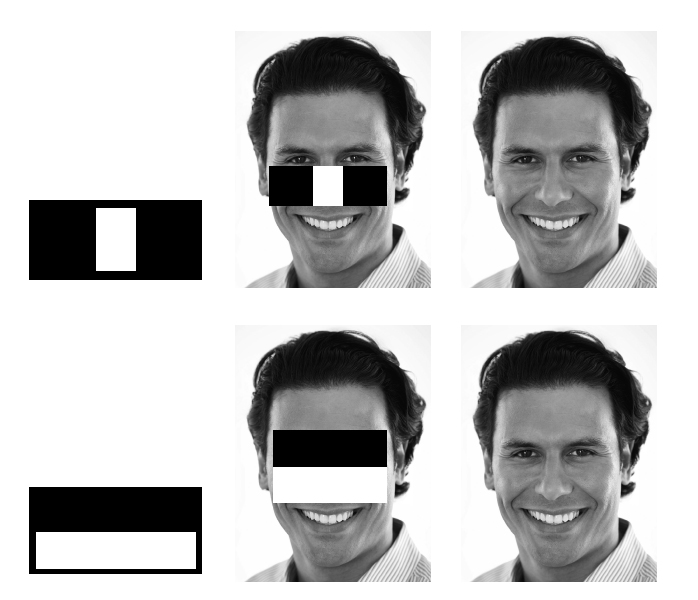
Figure 2. Haar-like patterns of light and dark rectangles can be fitted to facial images.
Whatever the algorithm, the feature extractor’s job is to produce a list of the features in the image, often with additional attributes about each feature. This list gets sent deeper into the pipeline for pattern recognition.
Getting Objects
The next stages in the vision pipeline will organize the extracted features into patterns that seem to have stable associations, and then to infer from those patterns of features the existence of objects in the scene. For example, in optical character readers, a group of strokes that are connected–or nearer to each other than to any other strokes–probably constitutes a character.
The challenge of binding together features to form objects becomes much more formidable in systems working with continuous-tone images such as photographs or video. These systems may take several successive layers of pattern extraction, attempting to group features by proximity, color, surrounding edges, or other rules suggested by a-priori knowledge of the subject. Once features have been grouped into patterns, the system often must apply further rules to identify patterns of features with objects. Or the system may use trained convolutional neural network layers to find patterns and infer objects.
For many systems, just locating objects, without any attempt to classify them, is sufficient. Two papers from the Embedded Vision Summit illustrate this point: a talk by Videantis vice president for marketing Marco Jacobs on single-camera 3D vision, and a keynote by Dyson electronics lead Mike Aldred on his company’s vision-driven robot vacuum, the 360 Eye.
Jacobs explained that algorithm developer Viscoda produced the 3D approach, which Videantis then adapted to their own single-instruction, multiple-data vision-processing chip. Rather than isolating objects and then measuring the distance to them, the algorithm identifies distinctive features in a scene—a cloud of feature points, Jacobs called them—through a series of matrix operations based on pixel-value gradients. By finding pixels where the gradient change is greatest, the algorithm basically acts as a corner detector.
The algorithm performs the extraction a second time on an image captured after the camera has moved a little. By comparing the locations of the feature points in the two images, the algorithm figures out which feature points match up between the two images, and develops motion vectors, not unlike the motion vectors used in video compression. A statistical solver uses these vectors to estimate camera motion, distance to each feature point, and motion that can’t be accounted for by parallax, and therefore must represent moving of the objects on which the features points lie.
“There is a lot of ambiguity in identifying feature points between frames,” Jacobs said. “So you want a cloud of around 1,000 to 1,500 feature points to get a good idea of the ranges to objects.”
Aldred described a similar approach used on the 360 Eye. He explained that once Dyson decided to create a robot, a simple reality almost dictated a vision-based system. Dyson’s signature centrifugal vacuum cleaner requires a powerful, high-rpm motor. “That gave us 45 minutes of battery life to do the vacuuming and get back to the charging station,” Aldred related. “So we couldn’t do a random walk—we had to build an accurate map and cover it methodically.”
The developers chose a vertically-mounted camera and a ring-shaped lens, producing a 360-degree image that reaches from the floor around the 360 Eye to well up the walls of the room. “There’s not much useful information on the ceilings of most rooms,” Aldred pointed out.
Using an approach similar to Viscoda’s, the Dyson vision processor populates this cylindrical surface with distinctive feature points. “It takes a very rich feature set,” Aldred observed. “The robot would not do well in an empty room with bare walls.” From consecutive images the system computes motion vectors, extracts objects, and performs simultaneous localization and mapping (SLAM) using Kalman filters.
Aldred reported that by far the longest process in developing 360 Eye has been testing and refining the algorithms. “The ideas were formed in 2008,” he said. “We proved out the maths in simulation, with recordings of real-world data—extensive real-world data—continuously developing the simulator as we progressed. But we also did in-home tests. Over eight years we’ve done 100,000 runs.”
Calling on Neurons
An enormous amount of testing is the price of rule-based algorithms. Unless you can constrain the environment so tightly that you can enumerate all possible situations, you face the chance that your rules will encounter a new situation and do something undesirable. This open-ended risk has led some researchers to revive an older approach to poorly-defined problems: neural networks.
Unlike systems that apply predefined mathematical functions and classification rules to images to extract features, identify and classify objects, and create predictive models, neural networks are simply consecutive layers of arrays of nodes—called, by analogy to biology, neurons. The output of each neuron at time t+1 is a function—usually non-linear and sometimes slightly randomized—of the outputs of some (or all) of the neurons in the previous layer at time t (Figure 3).
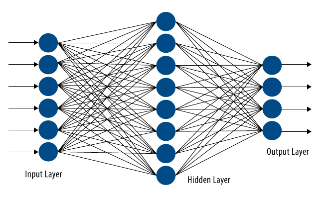
Figure 3. Neural network models connect all of the outputs of the previous layer to inputs of each neuron in the present layer.
Rather than choosing the input function for each neuron, you use a directed search process to train the neural network. In essence, after deciding the general kind of function you want each neuron to perform, you randomize all the parameters in all the neuron functions, present the first layer of the network with an image, and see how close the network comes to correctly classifying the image. For example, one output of the final stage of the network might indicate the presence or absence of a lion in the image. You measure the error between the actual network output and the correct classification, and then use that error to adjust the function parameters through the network in a direction that reduces the error. And repeat—over an enormous number of training images.
Neural networks were first tried for vision processing decades ago. But two problems stymied progress. First, as the image resolution increased, the number of neurons and connections exploded. Second, as the network grew, training times became intolerably long.
But two advances have relieved these problems. The first is the emergence of convolutional neural networks (CNNs). CNNs replace the neurons in the first few layers with small convolution engines. Where each neuron might be connected to a very large number of pixels or inputs from the previous layer, the convolution engines take as input only a small number of signals—a 16-by-16 array of pixels, for example. And instead of an arbitrary function that must be trained, the convolution engine does only one thing: it convolves its inputs with a kernel. You only have to use training to establish the values in the kernel.
One measure of the importance of CNNs comes from an industry benchmark, the Imagenet Large-Scale Visual Recognition open challenge, sponsored by a group of interested researchers that includes Facebook, Google, Stanford University, and the University of North Carolina. This large set of test images, accompanied by an even larger set of training images, has become the standard by which still-image recognition systems are measured.
CNNs have quickly dominated the Imagenet challenge, producing far more accurate object classifications than rule-based systems. But the training process to achieve these results can be enormous.
Ren Wu, distinguished scientist at the Baidu Institute of Deep Learning, described in a keynote how his organization has taken the lead in Imagenet challenge results, at least for the moment, with a misclassification rate of only 4.58 percent. To achieve that rate, Baidu uses a 16-layer CNN in which only the final three or four layers are made up of fully-connected neurons.
But the real effort goes into the training. Baidu has expanded the already exhaustive set of training images by generating variants of the Imagenet training set, varying the color and lighting and introducing optical distortions. The result is a set of about two billion training images—a seemingly impossible task for even a supercomputer-based CNN model to digest.
That brings up the second advance—hardware acceleration. The Baidu CNN is implemented on a custom supercomputer. During training, the system uses a stochastic gradient descent algorithm to refine the convolution kernels and neuron input functions. While the CNN model itself apparently runs on CPUs, the training algorithm executes on a bank of 32 Nvidia Tesla graphics processing units (GPUs), linked on a private Infiniband network.
Once the training is done, the computing load for executing the CNN model drops significantly. Wu said that you can use the full, trained CNN to train a smaller CNN quite quickly. It is possible in this way to get good performance on even very small devices. “Even a cell phone can run the trained model if you unpack the power of its GPU core,” Wu claimed. “We have a demo of an OpenCL™ model running autonomously on a smart phone, using the handset’s Imagination Technology GPU.”
IBM, meanwhile, is taking a quite different approach to hardware acceleration. Rather than execute CNN models on heterogeneous CPU/GPU systems, IBM’s TrueNorth program is staying with fully-connected neural networks but executing the models on an array of custom chips that directly emulate axons, synapses, and neuron cells.
The current chip packs the equivalent of a million neurons, with 256 million potential synaptic connections, onto each die. The full computer is a vast array of these chips connected through a network that allows an axon from any neuron to connect to a synapse of any other neuron. The behavior and threshold of each synapse is programmable, as is the behavior of each neuron. IBM has sown that the system is flexible enough to emulate any of the documented behaviors of biological neurons.
Aside from being fully connected and very flexible, the TrueNorth design has another important characteristic. Unlike models executing on stored-program CPUs, the neuron chip operates at relatively low frequencies, using quite simple internal operations. This allows a single chip to run on 100 mW, making mobile devices entirely feasible even with the existing 45 nm silicon-on-insulator process.
TrueNorth models can either be programmed with predetermined functions, or they can be architected and then trained with conventional back-propagation techniques. Using the latter approach, IBM researchers have demonstrated quite impressive results at classifying scenes.
We have examined a spectrum of vision-processing systems, each occupying some portion of the continuum from feature extraction to object classification to execution of predictive models. We have noted that along that continuum implementations tend to start out with simple mathematics for extracting features, then move to either complex rule-based classifiers and Kalman filters or to neural network models. And we have carefully avoided predicting whether neural networks and CNNs will turn out to be the preferred implementations of these challenging systems in the future, or will turn out to be a promising dead end.
By Ron Wilson
Editor-in-Chief, Altera Corporation