This article was originally published at CEVA's website. It is reprinted here with the permission of CEVA.
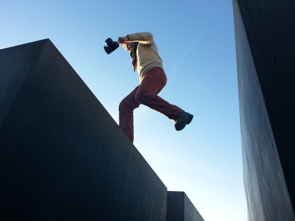
Demand is on the rise for video cameras on moving platforms. Smartphones, wearable devices, cars, and drones are all increasingly employing video cameras with higher resolution and higher frames rates. In all of these cases, the captured video tends to suffer from shaky global motion and rolling shutter distortion, making stabilization a necessity.
Integrating an embedded video stabilization solution into the imaging pipeline of a product adds significant value to the customer. It improves the overall video quality and, at the same time, enables better video compression and more robust object recognition for higher-level computer vision tasks.
Recently, we shared a brief technical overview of CEVA’s software-based stabilization solution. In that overview, we discussed the importance of video stabilization and the challenges presented throughout the development process in terms of accuracy, performance, and power. We also looked at how CEVA’s algorithm flow addressed all of these issues.
Today, we will take a deeper look inside, focusing on computer-vision-based video stabilization approaches. This series of two posts will explore trade-offs between factors, such as video quality and computation requirements, and reveal some insights from our years of experience.
Stabilizer Challenges
A number of challenges need to be addressed to reach a good stabilization solution.
First of all, the solution must be adaptive, and perform well in various scenarios: walking or running while holding a smartphone device, capturing video from a camera installed inside a car, or recording videos from drone devices. Collecting a rich test set that covers all of these motion types is an essential step when developing stabilization software.
The second challenge is to discriminate between desired and undesired motion. We need to keep only the motion intended to be captured, and remove any unwanted vibrations and distortions. These vibrations and distortions are usually caused by the camera internal system (for example, rolling shutter mechanism for CMOS sensors) and the way the camera is carried (for example, handheld or installed in a car or a drone). To accurately estimate and correct this complex motion, a six-axes camera motion model (x, y, z, pitch, roll, and yaw) is required at both the estimation and correction stages. This type of model usually requires more input data and consumes more power and CPU load.
With the growth in video quality, a good solution must also be able to handle high data rates of up to 4K resolution and 60 frames per second (fps). All of this must be achieved while keeping the power low, so that it can be used for embedded applications. On a system level, for example, we can achieve a low-power solution by joining together bandwidth-consuming stages like pyramid creation and feature detection stages. Working on multiple features together (in Scatter-Gather mode) can reduce the overhead and give much better kernel optimization (this will be explained later on).
Stabilizer Technologies
The two main strategies currently used to stabilize video are mechanical (referred to as Optical Image Stabilization (OIS)) and digital (referred to as Electronic Image Stabilization (EIS) or Digital Video Stabilization (DVS)).
The strengths of OIS are that it reduces motion blur, makes corrections based on the true camera motion, and minimizes high-frequency vibrations. The drawbacks of this approach, though, are high cost, high power consumption, additional components inside the camera, and limited motion range and degrees of freedom (DoF) due to the mechanical system structure.
The strengths of EIS are that it minimizes low-mid frequency vibrations, corrects complex and large motion ranges, and has a high level of flexibility, low power consumption, and a very low cost. This strategy also has its drawbacks: it has limited ability to reduce motion blur and it estimates the camera motion only from visual cues (as opposed to OIS, which is based on the true camera motion).
While each of these strategies has its strengths and drawbacks, the low power, low cost, and flexibility of the digital EIS approach make it a much better fit for the mass market. This is especially true for lightweight, portable devices that must be power efficient. From here on in, we’ll be looking at the digital approach, using computer vision for stabilization.
Video Stabilization Using Computer Vision
Video stabilization breaks down into two main parts: camera motion estimation and camera motion correction. Each of these parts has three stages:
- The estimation stages are feature detection, feature tracking or matching, and motion model estimation.
- The correction stages are motion smoothing, rolling shutter correction, and frame warping.
Our experience has taught us how to get the best results from each stage. In this post, we will share some insights about the first two stages.
Feature detection
Our first challenge is selecting the best-fitting feature detector. There are a wide variety of detectors, for example, Harris-Corner, Shi-Thomas, FAST, and Differences of Gaussians (DoG), to name a few. So how do we select the best one? To answer that, we need to look at the properties required for good detection.
In our experience, the most important requirements are selectivity, repeatability, sensitivity, and invariance.
- Selectivity is the algorithm’s ability to respond to corners and not to edges. Having good selectivity is crucial for robust feature tracking.
- The next requirement is repeatability, in other words, getting a consistent response for different frames. Repeatability is essential for successful feature matching.
- Next is the sensitivity of the detector. We want the detector to be sensitive enough to cover the entire frame with features but not too sensitive; otherwise, we will get responses on edges or even on noise. This property is critical for accurate global motion estimation.
- Finally, we need invariance under translation, rotation, scaling, and depth changes.
Understanding these requirements and how to tune the detector to achieve them, as well as selecting the right features for the next stage, is paramount to the overall success of the stabilizer.
Tracking/matching
For feature tracking, we use the Kanade-Lucas-Tomasi (KLT) algorithm. The advantages of this algorithm are that it is accurate, local, and gives a continuous response. On the other hand, it is prone to failure on large motion and illumination changes. To combat this, the range of motion can be expanded by using a scale pyramid, as shown in the figure below. To optimize performance, this pyramid can be created during the feature detection phase.
It’s important to take into account that there is a trade-off between the track length (that is, the number of frames a feature “lives”) and frame spatial coverage. If we want to lean towards track length, we will prefer strong features that last longer. But if we want to favor frame coverage, we will prefer weak but well-distributed features.
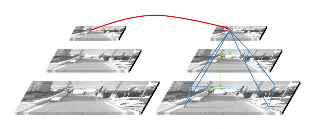
Figure 1: Coarse-to-fine optical flow using a scale pyramid
Feature matching is implemented using binary descriptors like BRIEF or FREAK. The advantages here are that it handles arbitrarily large motions, and has good invariance under illumination and geometric changes. Its main disadvantage is that it doesn’t do very well with repetitive textures.
Let’s take the figure below as an example. Feature matches from two frames are printed on the image. We can clearly see that the upper part is rich with matches (some of them are noisy but most of them are valid), but the lower part doesn’t have any matches at all. This can be explained by the way the feature matcher works: to increase confidence and reduce ambiguity, if the matcher gets more than two features with similar descriptors, it removes them all. Because the floor in this picture has repetitive textures, all of the features share almost the same descriptors, and so they are all removed by the matching process.
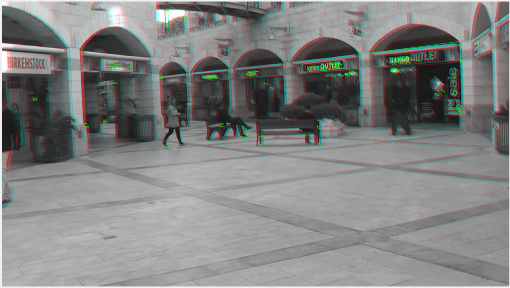
Figure 2: Binary matching results for an image with repetitive textures
To accelerate the process, we can filter candidates for feature matching. The filter could be based on location, scale, or orientation. Another method of acceleration is to use inertial sensor data as a coarse prediction for the location of the features in the next frame.
In embedded devices, feature tracking and matching must be extremely efficient. A good embedded solution should exploit data parallelism using Single Instruction Multiple Data (SIMD) operations. Instead of working in a patch-by-patch mode, we use Scatter-Gather mode to optimize the kernel. In this mode, multiple patches are loaded from random places throughout the image and processed together on the same cycles. This method dramatically boosts performance by reducing the number of function calls and minimizing the overhead of entering and exiting the internal loop.
We use dedicated operations for parallel convolution, and parallel arithmetic operations to process data from different patches on the same cycle. By using fixed-point implementation, we can achieve even better performance while the accuracy is still good enough for video stabilization.
In the next post, we will take a look at the motion model estimation and the motion correction stages. In the meantime, check out our DVS demos. Or, find out more about CEVA’s DVS solutions by clicking here.
By Ben Weiss
Imaging and Computer Vision Developer, CEVA