This blog post was originally published at Au-Zone Technologies’ website. It is reprinted here with the permission of Au-Zone Technologies.
The introduction of low cost, powerful Arm processors coupled with the advances in machine learning techniques provides the foundation for intelligent computer vision edge devices. Computer vision at the edge will drive the shift from cloud-centric intelligence to edge intelligence for many use-cases as edge devices offer many advantages. For example, edge video processing can provide deterministic response times, reduced network bandwidth costs, and increased data protection just to name a few. Object detection and tracking are the initial use-cases for which the momentum to shift to edge-based solutions is gaining speed. However; there are plenty of pitfalls developers must avoid to successfully navigate the design challenges associated with computer vision and machine learning. Understanding the design challenges and design trade-offs can reduce risk and accelerate time to market. Let’s take a look at a recent object tracking project we did.
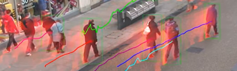
For this object tracking use-case we implemented a vision system for the measurements of customer service in a retail setting. The goal of the system is to measure the checkout time and number of customers who have been served in each lane as shown below in figure 1. To determine these customer analytics from the live video feed, we need an understanding of the position and movement of the individual customers as they pass through the field of view.
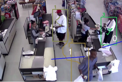
Figure 1 Customer tracking and counting
Many practical applications require a combination of traditional computer vision algorithms and machine learning techniques for the efficient implementation on a resource constrained edge processor. The advantage of this technique is that the object detector can provide interpolation of the object locations between detections as well as offering the context of the motion. The interpolation increases the effective processing frame rate allowing it to fill the gaps between detection frames, which is limited by longer latencies on the embedded platform. The design goal for this example was to process two checkout lines in real time running on an embedded Raspberry Pi processor.
The high-level block diagram of the implementation is shown below in Figure 2. After the image is captured an SSD object detector is used to find the initial positions of customers. Object detection was accomplished using a MobileNet V3 SSD model that was trained, tested and converted for target execution using the DeepViewTMML Toolkit. The obvious goal for object detection is high enough accuracy to meet the requirements of the application while still meeting the real time performance requirements. The DeepViewML Tools and optimized DeepViewRT inference engine greatly simplify the process of selecting, training and validating the appropriately sized detection model for standard or custom classes. For this particular use case a MobileNet V3 small network gave the best tradeoff of performance and accuracy with an inference time of 145ms.
Once the object has been detected the bounding box is sent to a configurable tracker which is used to calculate the path of the object as it moves within the field of view. For this example, a tracker was implemented using a Kernelized Correlation Filter (KCF). The kernel function is used to calculate the similarity between the tracked target and shifted candidate area which is less computationally intensive than detection. The goal here is determined where the object has moved so tracking must be performed at a reasonable frame rate compared to the speed of the object. In this implementation the KCF tracker runs in less than 50ms which enables higher speed processing compared to detector only based algorithms.
To improve the robustness of the tracking algorithm other state machines and filters may be used to deal with situations such as occlusion where that path of the object is blocked by another object over a portion of the field of view. A Kalman filter is used to predict the object state based on the previous direction and speed of the object when good correlation from the tracker is not obtained. The Kalman Filter can also filter out the outliers to improve the state Signal-To-Noise Ratio.
The key steps for Kalman Filters are a) Object Prediction and b) Bounding Box Correction. The Object Prediction phase uses a dynamic model that defines a velocity vector which can be used to estimate the object’s future position. During the Bounding Box Correction Phase, the bounding box from the Prediction Phase is compared to the location as determined by the tracking algorithm to estimate a posterior bounding box. The posterior bounding box will be located in-between the predicted and measured bounding box. The updated location of the object will thus be determined to be the measured location if the object detector’s confidence is high; or it will be the posterior location if the detector’s confidence is low. If the object detector fails, the predicted location will be used. Kalman Filters for location prediction are used in-between the nth frames that are processed by the Object Detector.
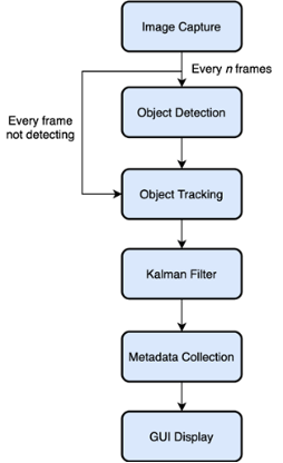
Figure 2 Object Detection and Tracking Flow Diagram
After a configurable number of tracking frames detection is performed again to confirm the tracked location. It is then necessary to determine if the detected object is the same as the object which is being tracked, which is an assignment problem. The Hungarian algorithm is used to integrate the results from tracker, new detections, and predictions. The Hungarian algorithm can determine if the object in two frames is the same, this can be based on intersection over union (IOU), shape of the object, or convolution features. Threshold values are established, and if met, the object is concluded to be the same.
Once we can track objects, the next step is to collect data on each object’s movement. A straightforward approach is to determine the path of the object using the history of the object’s previous centroid locations as in Figure 3. This data can then be used to visualize movement in an application or determine if an object has intersected a boundary line or zone.
Figure 3 History of Centroids
The final software architecture for the solution is shown below in Figure 4. The input video is scaled by the camera server for appropriate resolution for the object detector and tracker algorithms. Metadata from the tracking algorithm is processed by the application which generates the bounding boxes and paths on the display in real time along with the number of customers served for each lane and the service timing.
The solution has the following tunable parameters so that it can be set up and optimized for other uses cases:
- Detection Rate: the number of milliseconds between each detection
- Model Type: the type of ML model used for object detection
- Tracker: the tracking algorithm used
- Object minimum size: minimum size of object to track
- Object maximum size: maximum size of object to track
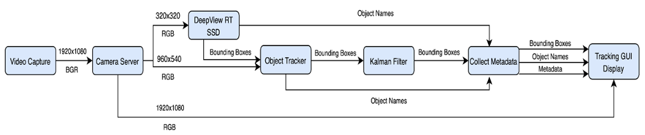
Figure 4 The Final Architecture
With this implementation we were able to show a practical tracking solution capable of processing two checkout lanes in real time running on an embedded Raspberry Pi4 platform. A demo video of the working solution is available here.
Brad Scott
Co-founder and President, Au-Zone Technologies