This article was originally published at Au-Zone Technologies’ website. It is reprinted here with the permission of Au-Zone Technologies.
Unlike image classifiers, which simply report on the most important objects within an image, object detectors determine where objects of interest are located, their sizes and class labels within an image. Consequently, object detectors are central to numerous computer vision applications.
In this article, we provide a technical introduction to deep-neural-network-based object detectors. We explain how these algorithms work, and how they have evolved in recent years, utilizing examples of popular object detectors. We will discuss some of the trade-offs to consider when selecting an object detector for an application, and touch on accuracy measurement. We also discuss performance comparison among the models discussed in this article.
Early Approaches
The seminal work in this regard was reported in the form of technical report at UC Berkeley, in 2014 by Ross Girshick et al. entitled “Rich feature hierarchies for accurate object detection and semantic segmentation”. This is popularly known as “R-CNN” (Regions with CNN features). They approached this problem in a methodical way with having 3 distinct algorithmic stages which is shown in Figure 1 below.
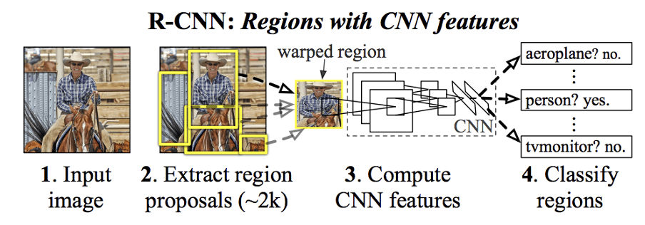
Figure 1: R-CNN [“Rich feature hierarchies for accurate object detection and semantic segmentation”]
As seen above, there are three stages:
- Region Proposal: Generate and extract category independent region proposals, using selective search.
- Feature Extractor: Extract feature from each candidate region using a deep CNN
- Classifier. Classify features as one of the known classes using linear SVM classifier model.
Here the main issue was that it produces lots of overlapping bounding boxes and post processing and filtering was needed to produce reliable results. Consequently, it was very slow and require 3 different algorithms to work in tandem. A faster version of this approach was published in 2015 entitled “Fast R-CNN” where authors combined second and third stages into one network with two outputs – one for classification and the other for bounding-box regression.
Shortly afterwards, they published “Faster R-CNN: Towards Real-Time Object Detection with Region Proposal Networks” where region proposal scheme was also implemented using a separate neural network.
Recent Approaches
YOLO
In 2016 a mark departure was proposed by Joseph Redmon et al. entitled “You Only Look Once: Unified, Real-Time Object Detection” or in short, YOLO. It divides the input image into an S × S grid. If the centre of an object falls into a grid cell, that grid cell is responsible for detecting that object. Each grid cell predicts B bounding boxes, confidence for those boxes, and C class probabilities. The Figure 2 below shows the basic idea.

Figure 2: YOLO [You Only Look Once: Unified, Real-Time Object Detection]
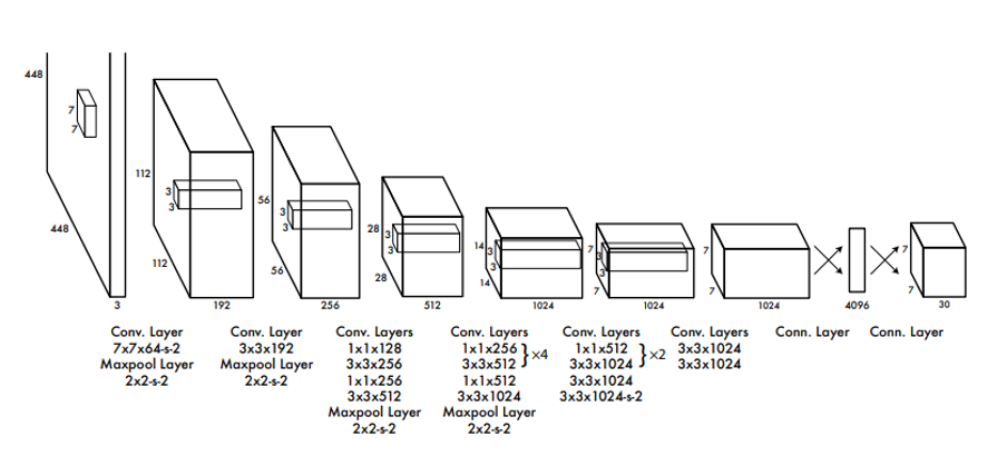
Figure 3 below shows the network architecture for YOLO detector. The network has 24 convolutional layers followed by 2 fully connected layers. Alternating 1 × 1 layers reduce the features space from preceding layers. The convolutional layers were pretrained on the ImageNet classification task.

Figure 3:YOLO Network Architecture
The predictions are encoded as an S × S × (B ∗ 5 + C) tensor. YOLO imposes strong spatial constraints on bounding box predictions since each grid cell only predicts two boxes. It can only have one class in a cell. This model struggles with small objects that appear in groups, such as flocks of birds.
YOLO-v3 was proposed in 2018 which utilizes multi-resolution approach with three different grid sizes 8×8, 16×16 and 32×32. Objects were learned based on the resolution and anchors. Each resolution has at least 3 anchors to define objects ratios at each cell.
Recently, in 2021 YOLOX was proposed which is anchor free and utilized decoupled output heads for class labels, bounding box regression and IoU, as shown in Figure 4 below.

Figure 4: YOLOX
SSD (Single Shot Detector)
This approach evaluates a small set of default boxes of different aspect ratios (anchor boxes) at each location in several feature maps with different scales (8 × 8 and 4 × 4 in (b) and (c) in Figure 5 below).
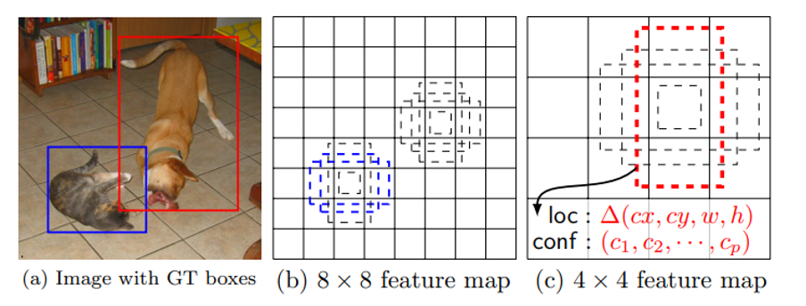
Figure 5: [SSD: Single Shot MultiBox Detector]
The SSD model adds several “feature scaler layers” to the end of a backbone network, which predict the offsets to default boxes of different scales and aspect ratios and their associated confidences. The figure below highlights the differences between YOLO and SSD. For each default box, it predicts both the shape offsets and the confidences for all object categories.

Figure 6: SSD vs YOLO
Inference frame rate (speed with batch size 8 using Titan X and cuDNN v4 with Intel Xeon [email protected].) is 46 fps for SSD of 300×300 pixel images with mAP = 74.3%. Whereas for YOLO (VGG-16) frame rate is 21 fps of 448×448 pixel images with mAP=66.4%. For SSD, output candidate bounding boxes can be very large (~8732) therefore Non-Maxima Suppression (NMS) post-processing needs to be optimized.
RetinaNet
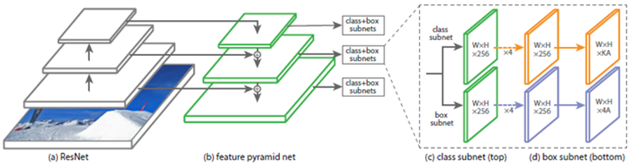
Figure 7: [Focal Loss for Dense Object Detection]
This technique utilizes Feature Pyramid Network (FPN) backbone on top of feedforward ResNet architecture. They introduced Focal Loss to handle class imbalance in object detection dataset.
RetinaNet with ResNet-101-FPN matches the accuracy of ResNet- 101-FPN Faster R-CNN. The inference time is 172 msec per image on nVidia M40 GPU.
CenterNet
In 2019 CenterNet was proposed which had very different approach as compared to other object detection techniques discussed so far. It is trained to produce gaussian blob (heatmaps) at the centre of the object, thereby eliminating the need for anchor boxes as well as NMS post filtering.
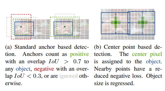
Figure 8:[Objects as Points]
Object are localized by detecting the local maxima from the heatmaps. Single network predicts the keypoints (local maxima of heatmaps), offset, and size. The network predicts a total of C + 4 outputs at each location.
CenterNet is not the best in terms of accuracy but provides excellent accuracy-speed trade-offs. It can easily be extended to 3D object detection, multi-object tracking and pose estimation etc.
Evaluation Framework – Accuracy Measurement
True Positive (TP) — Correct detection made by the model.
False Positive (FP) — Incorrect detection made by the detector.
False Negative (FN) — A Ground-truth missed (not detected) by the object detector.
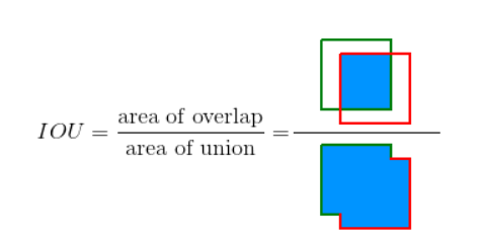
Intersection over Union (IoU)
The IoU metric in object detection evaluates the degree of overlap between the ground (gt) truth and predicted (pd) bounding boxes. It is calculated as follows:
IoU ranges between 0 and 1, where 0 shows no overlap and 1 means perfect overlap between ground truth and predictions.
IoU is used as a threshold (say, α), and using this threshold one can decide if a detection is correct or not. Consequently:
True Positive (TP) is a detection for which IoU(gt,pd)≥ α
False Positive (FP) is a detection for which IoU(gt,pd)< α
False Negative (FN) is a ground-truth missed with gt for which IoU(gt,pd)< α
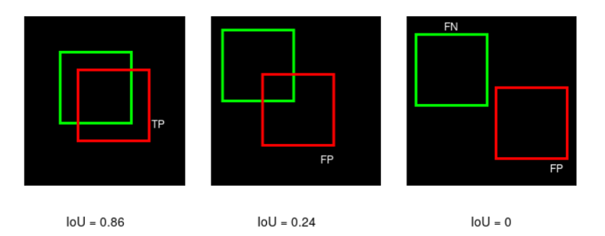
If we consider IoU threshold, α = 0.5 , then TP, FP and FNs can be identified as shown in the Figure above. If we raise IoU threshold above 0.86, the first instance will be a FP and if we lower IoU threshold below 0.24, the second instance becomes TP.
Precision is the degree of exactness of the model in identifying only relevant objects. It is the ratio of TPs over all detections made by the model.
Recall measures the ability of the model to detect all ground truths—TPs among all ground truths.
A good model is supposed to have high precision and high recall.

Raising the IoU threshold means that more objects will be missed by the model (more FNs and therefore low recall and high precision). Conversely, a low IoU threshold will mean that the model gets more FPs (hence low precision and high recall).
The precision-recall (PR) curve is a plot of precision and recall at varying values of IoU thresholds. As shown in the figures below, the P-R curve is not monotonic, therefore smoothing is applied.
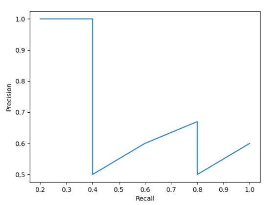
Figure 9: Precision-Recall Curve

Figure 10: Precision-Recall Curve (smoothed)
Average Precision (AP)
AP@α is Area Under the Precision-Recall Curve(AUC-PR) evaluated at α IoU threshold. AP50 and AP75 mean AP calculated at IoU=0.5 and IoU=0.75, respectively.
Mean Average Precision (mAP)
There are as many AP values as the number of classes. These AP values are averaged to obtain the metric – mean Average Precision (mAP). Pascal VOC benchmark requires computing AP at 11 points – AP@[0, 0.1, …, 1.0]. MS COCO describes 12 evaluation metrics shown below.

Comparisons
In this section we summarize and present comparisons which are published in the publicly available research papers.

The table above provides comparisons between SSD, YOLO and others on PASCAL VOC 2017 dataset. The tests were done on Titan X GPU and cuDNN v4 with Intel Xeon [email protected].
Here we see that SSD model is faster with higher mAP but produces lots of boxes and therefore decoding and NMS post filtering can be time consuming.
The table below provides comparison for RetinaNet with others on MS COCO dataset. Here RetinaNet with ResNet-101-FPN and a 600×600 pixel image size (on nVidia M40 GPU) runs at 122 msec per image. It shows that RetinaNet can good very good accuracy with ResNext-101-FPN backbone.

The next table below provides comparisons with CenterNet and the previous detectors on COCO dataset. The tests were performed with Intel Core i7-8086K CPU, Titan Xp GPU, Pytorch 0.4.1, CUDA 9.0 and CUDNN 7.1.

Here it can be observed that CenterNet gives best tradeoff between FPS and accuracy.
Choosing An Object Detector
There is no single best detector and choosing one involves looking several factors including application and hardware requirements. In general, highly accurate models are more complex and of larger sizes making them unattractive for embedded or resource constrained devices. On the other hand, smaller models tend to be faster but less accurate. Model size can be reduced, and inference speed can be enhanced using quantization from 32-bit floats to 16-bit floats or 8-bit integers. Obviously, significant boost in speed can be achieved on dedicated hardware such as GPU, NPU etc. at the expense of portability. The table below provides general observations when it comes to deployment.
| Model Type | Accuracy | Speed | Size | Portability |
| FP-32 bit natively trained | Highest | Lowest | Largest | High |
| FP 16 | Low | Low | Small | Medium |
| Int 8, Int 16 | Lower | Fast | Smaller | Low |
| Compute Unit | Lower | Fastest | Small | Low |
Challenges On Edge Devices
In earlier sections we established some guidelines about Object Detection algorithms as well as pros and cons. To select the model that fits best for a given problem is a challenging task when working on edge devices. Most of the time, the objective is to maximise the accuracy as much as possible while maintaining a low inference workload and timing. The problem is that these are often conflicting requirements when compute resources are constrained or fixed as shown in the diagram below.

Training on detectors with custom datasets with eIQ
Usually, selected models should be fine-tuned or retrained on custom dataset without having clues about the generalization level. The end goal is the model learns to generalize as much as possible real-world images after seeing training samples. This point constitutes a challenge by itself given the vast number of parameters the model must train. On the other hand, there are few external parameters that play important roles within the training process, commonly known as hyper parameters. Hyper parameters involve learning rate, batch size, epochs, decay, etc. Since the training process oversees tuning millions of parameters we need to be carefully when selecting these hyper parameters because that could be the difference in having successfully training sessions or not. Along with the hyper parameters, we need good initialization values, so our model learns to generalize in custom dataset as faster as possible. If initialization values are not properly set, we could have undesirable situations like overfitting or poor generalization.
Deploying trained detectors to embedded platforms
Before deploying any model on any embedded platforms, it is important to have a well-defined and widely tested pipeline, otherwise compatibility problems, memory errors and issues related to unsupported ops could arise. Additionally, a deep understanding on the model architecture as well as in Machine Learning might be required to modify models and make them able to run on the edge devices.
Unlike classification, object detection algorithms return raw predictions that need to be decoded for specific functions. In most of the cases these functions do not have a side-by-side support on embedded platforms libraries. Quantization support is not always fully achievable in all the models, which make them to run in mixed precisions, some ops run on low bits (uint8, int8) while the rest run on (float16, float32). Even when this characteristic is not a big problem, to have the full model running in low bits (uint8, int8) always improve timings, and reduce memory and energy consumption.
To mitigate the impact of these common problems encountered when performing object detection at the edge, eIQ Portal provides a set of tools to handle these issues for embedded developer. These tools are integrated within easy-to-use GUI for quick and transparent execution – thereby reducing trial and error steps in the process. Complex concepts like data annotation, data augmentation, training a model (classification or detection), model evaluation on targets devices and model deployment are transformed into GUI components so the normal user does not have to deal with all the intricacies of training and deploying AI models on target hardware.
Conclusions
In this blog we introduced early DNN-based object detectors, R-CNN, Fast R-CNN, Faster R-CNN. The recent ones include YOLO, YOLOX, SSD, RetinaNet and CenterNet. We introduced object detection error types, precision-recall curve as well details of computation of mAP. We discussed performance and speed comparisons mentioned in the literature along with our own (@Au-Zone) inference performance on in-house dataset on iMx8mPlus HW. Finally, we provided general guidelines and factors involved in choosing object detectors. We will be following up on this post with Part II, which will provide details on real world performance for many common DNN based detection models on NXP processors including the i.MX8MPlus. i.MXRT1060 and i.MXRT1170.
Azhar Quddus, PhD.
Senior Computer Vision Engineer, Au-Zone Technologies
References
R-CNN
Ross Girshick Jeff Donahue Trevor Darrell Jitendra Malik, “Rich feature hierarchies for accurate object detection and semantic segmentation”, Tech report (v5), UC Berkeley, 2014
https://arxiv.org/pdf/1311.2524.pdf
Fast R-CNN
Ross Girshick, “Fast R-CNN”, Microsoft Research, 2015.
https://arxiv.org/pdf/1504.08083.pdf
Faster R-CNN
Shaoqing Ren, Kaiming He, Ross Girshick and Jian Sun, “Faster R-CNN: Towards Real-Time Object Detection with Region Proposal Networks”, Advances in Neural Information Processing Systems, 2015.
https://arxiv.org/pdf/1506.01497.pdf
YOLO-v1
Joseph Redmon, Santosh Divvalay, Ross Girshick, Ali Farhadiy, “You Only Look Once: Unified, Real-Time Object Detection”, 2015.
https://arxiv.org/pdf/1506.02640.pdf
YOLO-v3
Redmon, Joseph, and Ali Farhadi. “Yolov3: An incremental improvement.“, 2018.
https://arxiv.org/pdf/1804.02767.pdf
YOLO-v4
Bochkovskiy A, Wang CY, Liao HY. Yolov4: Optimal speed and accuracy of object detection, 2020.
https://arxiv.org/pdf/2004.10934.pdf
YOLOX
Zheng Ge, Songtao Liu, Feng Wang, Zeming Li, Jian Sun. YOLOX: Exceeding YOLO Series in 2021.
https://arxiv.org/pdf/2107.08430.pdf
SSD
Wei Liu, Dragomir Anguelov, Dumitru Erhan, Christian Szegedy, Scott Reed, Cheng-Yang Fu, Alexander C. Berg, “SSD: Single Shot MultiBox Detector“, 2015
https://arxiv.org/pdf/1512.02325.pdf
RetinaNet
Tsung-Yi Lin, Priya Goyal, Ross Girshick, Kaiming He, Piotr Dollár, “Focal Loss for Dense Object Detection”, 2017.
https://arxiv.org/pdf/1708.02002.pdf
CenterNet
Kaiwen Duan, Song Bai, Lingxi Xie, Honggang Qi, Qingming Huang, Qi Tian, “CenterNet: Keypoint Triplets for Object Detection”, 2019.
https://arxiv.org/pdf/1904.08189.pdf
Accuracy
Object Detection Metrics With Worked Example
https://towardsdatascience.com/on-object-detection-metrics-with-worked-example-216f173ed31e#:~:text=Average%20Precision%20(AP)%20and%20mean,COCO%20and%20PASCAL%20VOC%20challenges