This blog post was originally published at Tryolabs’ website. It is reprinted here with the permission of Tryolabs.
This is the third entry in our Road to Machine Learning series; if you read the first and second entries and did your homework, congratulations! The force is growing on you! By now, you should feel familiar with the basics of a Machine Learning project: Clean, Train, Measure/Visualize, and Repeat. If that is the case, you might be looking for something more challenging, something to impress your friends, wow your partner, or showcase in your LinkedIn profile.
If all these resonate with you, look no further. In this episode, we dive into one of the most popular Computer Vision types of problems that we encounter in our projects: object detection and tracking. We will follow a hands-on exercise and use modern tools from beginning to end. We will not delve into the details of deep learning, but we encourage you to do so! You may want to check these resources before starting the exercise to grasp the concepts we will use and make the most out of this post.
Course #1
- Arguably, the most popular and complete online course that many of our engineers have followed is Stanford’s CS231n. The 1, 2, and 3 are available online. Lectures from past editions are on YouTube.
Course #2
- Once again, Andrew Ng provides an excellent specialization for free and even gives you a certificate of completion
We will also offer some related technical posts of similar work we have done to give you a better idea of what is possible with these technologies.
MaskCam
Seeed
- We partnered with Seeed to detect if employees were using safety gear, such as helmets, on construction sites.
Norfair
- We even developed our own open-source library for object tracking Norfair (which just celebrated it’s second birthday with a new release!)
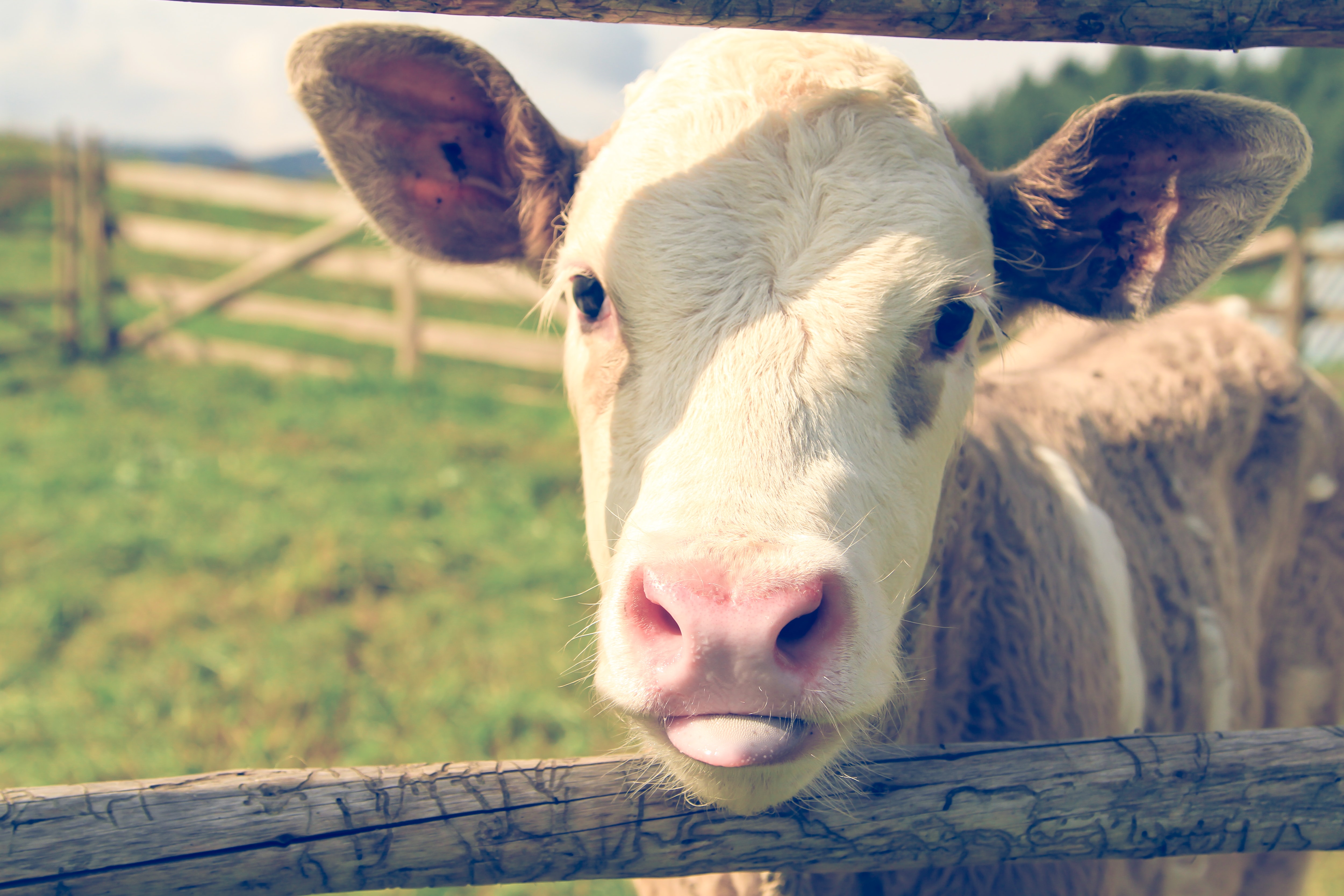
During this exercise, we will work with images and videos of one of the most adorable animals on earth: cows. They are second only to the internet overlords: cats and dogs. Beware, puns are going through the hoof for this blog post. Let’s see cow we do!
Hay there, my friend!
Introducing our Detection Box
For the sake of flow, we will take a top-down approach in which we ignore most of the technical details first and go back to them towards the end.
At a very general level, every Machine Learning project requires a model and a dataset. A Machine Learning model that performs object detection receives an image or video (you can think of videos as a sequence of images) as input and returns bounding boxes with all the objects identified. We will see an example of this shortly.
The architectures behind most object detection models are not complicated. However, they are not simple either. They involve using deep neural networks with several layers and loss functions.
For now, let’s treat the model as a Cowffee Machine (If you didn’t get that reference, go and read our previous blog post in the series.) Since all good things have a name, let’s call it DetectionBox.
An overview of our DetectionBox
To train a DetectionBox, we need ground truth, which consists of a set of images and their annotations in this context. An annotation is a collection of all the information we need to identify the information in the image. For classification, it is a single label. Yet, for object detection, it consists of a list of bounding boxes and a label for each box.
Training a detection object model from scratch is hard because it requires considerable data. But the vast majority of the time, we don’t train object detection models from scratch. Instead, we use a technique called transfer learning. In a nutshell, with transfer learning, we start from “pre-trained” DetectionBoxes that were trained once with a large dataset such as CoCo. In practice, it is even more involved than that. The pre-trained model is often pre-pre-trained with a pure image detection dataset such as ImageNet. We know, we know, that’s why we saved the details for last.
A DetectionBox only predicts items for the classes it has seen during training. If there are no unicorns in your dataset, even when presented with a unicorn, the model will not be able to find it. Fortunately, when we use transfer learning, we can alter the number of objects the model can predict.
Drawing the cowrtain
We said this blog post was a hands-on exercise, so without further ado, the exercise. But don’t get too excited yet! We know the feeling of getting familiar with new technology and the urge to try it right away and see how it goes. During the post, we will break down every step in this exercise and analyze what is happening.
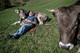
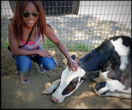
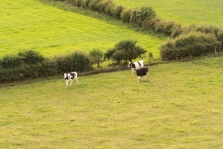
But first, let’s introduce our dataset cowtestants. We will use them as our testing dataset.
 |
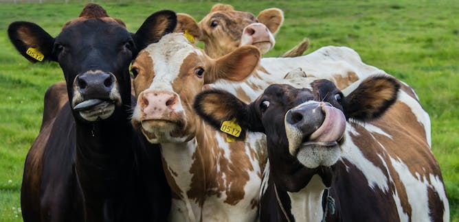 |
| Chilling and getting acowinted | Can you spot the little one in the back? |
Getting started
The beginning of every notebook looks very similar, install stuff, import what you installed, and define some helper functions. Let’s break it down.
The first two cells are for installing stuff we will need: pyyaml for reading YAML files, hub for downloading the annotated dataset, norfair to do object tracking, cowsay for the memes, jupyter_bbox_widget to draw bounding boxes on images, torchmetrics to make our lives easier when it comes to using metrics, and detectron2 for the trained models.
!python -m pip -q install pyyaml hub norfair cowsay jupyter_bbox_widget torchmetrics

# Detectron2 has not released pre-built binaries for the latest pytorch (https://github.com/facebookresearch/detectron2/issues/4053)

# so we install from source instead. This takes a few minutes.

!python -m pip -q install 'git+https://github.com/facebookresearch/detectron2.git'
The next cell, which we are omitting here for the sake of readability, contains a bunch of imports that we will use throughout the exercise.
Getting the hooves dirty
Now that we have finished with our configuration let’s dive into the most exciting parts of the exercise. You will now see a cell where we define our DetectorBox class which, once again we omit for the sake of readability. Don’t worry too much about this yet. The only thing you need to know to follow the post is that the class has three methods: predict, train, and evaluate.
class DetectorBox:

def __init__(self):

# here we instantiate the class

def predict(self, img, metadata=None, visualize=False):

# used to predict a single image

def train(self, dataset_name, epochs=500):

# method used to train the model

def evaluate(self, image_dict, metadata=None):

# method used to evaluate the performance of the model
What you will see next are the following cells:
# Download images from the internet

!mkdir -p internet_cows

!wget -q -A jpg 'https://encrypted-tbn0.gstatic.com/images?q=tbn:ANd9GcTPrhZZxQ0eMyBxx2Uqgu1z6p6p4jLhRrvNQg&usqp=CAU' -O internet_cows/0.jpg

!wget -q -A jpg 'https://images.theconversation.com/files/472297/original/file-20220704-12-7zgqd5.jpg?ixlib=rb-1.1.0&rect=0%2C220%2C3496%2C1748&q=45&auto=format&w=668&h=324&fit=crop' -O internet_cows/1.jpg
black_box = DetectorBox()

for pth in Path('internet_cows').glob("*.jpg"):

img = np.array(Image.open(pth).convert("RGB"))

pred = black_box.predict(img, visualize=True)
What just happened here? We instantiated our DetectorBox, downloaded the images from the internet, loaded the images using the pillow library (a classic library for image manipulation in Python), and fed the images to our model.
We can now turn our attention to the model’s output and see what we got for the first image… and it’s a dictionary !
preds[1]

{

"pred_classes": tensor([16, 0, 16, 16], device='cuda:0'),

"pred_boxes": Boxes(tensor([

[ 92.7439, 35.9965, 171.0376, 88.4358],

[ 36.1270, 33.2318, 134.8450, 136.7290],

[ 47.5423, 35.9811, 164.8269, 133.4164],

[ 39.0535, 25.4165, 99.2579, 88.4267]],

"scores": tensor([0.9733, 0.8099, 0.8042, 0.7629],

}
How do we interpret this? First, we see that we have four pred_classes, which means that our algorithm identified four “things.” But what are these? Those numbers: 16, 0, 16, and 0 indicate the class of each thing.
We need to take a step back here and explain something. Our DetectionBox was trained on a dataset with 91 classes: from cows to dogs and cars. That model only predicts things within those classes, and 16 and 0 are two of them.
Let’s keep on moving. The pred_boxes field indicates where those “things” are located. Each row is a set of coordinates: x_min, y_min, x_max, y_max, and those coordinates are in pixels! Finally, the score represents the model’s confidence when predicting the class.
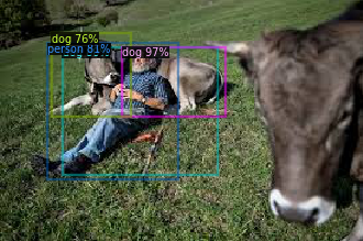
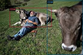
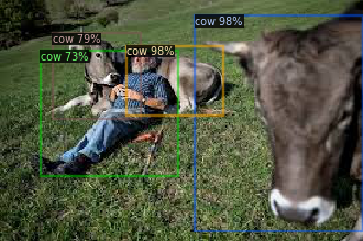
Now, in this format, it is cumbersome to understand if those predictions are okay. It would be much easier to see it. Luckily we already instructed Python to print these images with our visualize=True parameter:
 |
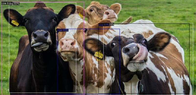 |
Now we have the boxes drawn on top of the image with the corresponding class and score. Can you spot the problem? Turns out that 0 = person and 16 = dog. Hence, the algorithm didn’t identify a single cow in the image on the left. And although we get some cows in the second image, those are not great either. Some dogs and some cows are not correctly “boxed.”
Improving our model
To improve our model, we need to do two things. On the one hand, we need to improve our model performance. On the other hand, we need to find a way to automatically “score” the predictions since inspecting thousands of images manually does not scale very well. To do this properly, we first need to annotate some images and then measure the results. Let’s start with the former.
Annotating images
To automatically assign a value to our prediction, we need to provide ground truths for each image. We will do that by “drawing” bounding boxes on top of them. This is a manual process because, unlike other types of data, it is almost impossible to start with data already annotated in the required format. (Who would draw bounding boxes for fun?)
Nowadays, several companies and software can be used to improve the annotation process. However, since we are learning, there is nothing like doing something yourself.
In a Jupyter Notebook, we can use a widget to draw as follows:
# Auxiliary function that encodes an image into base64 because this is

# what is needed by the jupyter_bbox_widget, the package we installed before:

preds[1]

def encode_image(filepath):

with open(filepath, 'rb') as f:

image_bytes = f.read()

encoded = str(base64.b64encode(image_bytes), 'utf-8')

return "data:image/jpg;base64," + encoded

widget_0 = BBoxWidget(

image=encode_image('internet_cows/0.jpg'),

classes=['cow']

)

widget_0
and get the coordinates:
coordiantes = widget_0.bboxes
After drawing the boxes, they should look something like this:
 |
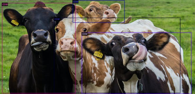 |
Drawing bounding boxes is not as straightforward as it might first sound. Let’s look at this example in particular. For the first image, we decided to draw the whole cow even though a person obstructed the view. In the second image, we selected only the face of the cow that appears behind all the others. This might cause problems because the algorithm learns that a cow is a cow head, a cow split into two, and a whole cow. We could decide only to annotate full cows, but we would miss a lot of the partially occluded ones. Also, we could tag heads only, but we would not know where the bodies are. There are no apparent answers to these questions. In our experience, the best way forward is to treat this as an iterative process: annotate some, manually inspect for errors, and attempt to understand if some of those are systematic. If they are, you can update the labels.
Scoring our predictions with metrics
The next question we want to tackle is how to formalize the process of checking if the model output is correct or not. Ideally, we could have a metric that summarizes how good the predicted bounding boxes are compared to the actual bounding boxes. The most popular metric in object detection problems is the Mean Average Precision (mAP).
For this blog post, we will assume that given a set of ground truth images and the predicted bounding boxes, we can obtain the mAP: a single score of how well the model performs in the given dataset. This score gives us a number between zero and one where zero is really bad, and one is perfection. We encourage you to learn more about this metric in this video.
mAP further reading
- If you are really curious about how this metric works, you can find a more in-depth explanation of this process in this blogpost and in this one.
If you want to know how we implemented this for this exercise, check out the method evaluation of our DetectorBox.
If we apply this metric to our current dataset of two images, we get a score of 0.1290, which is fairly low. Now that we have an objective metric of our model’s performance, let’s see how we can improve this score.
Transfer-learning & fine-tuning
One of the advantages of neural networks is that we can stop and resume training them at any point: even with different data. If you were using XGBoost, changing your dataset or updating it with new information is not easy and might require access to the original dataset and the new one. That’s not the case with neural networks. Simply get the new data and perform a few iterations. The weights (the parameters) evolve from the last “check point.”
This seemingly minor detail is actually crucial. We can use large public datasets to teach a model to recognize general patterns such as faces, objects, and more. Then, use a smaller dataset to teach it how to connect the information extracted about faces and objects in the context of the smaller dataset. This process is often called transfer learning or fine-tuning. This is the backbone of many Machine Learning projects, especially Computer Vision ones.
Interesting reads:
- Pytorch’s official fine-tuning guide for vision models.
The larger model using public data is often trained by large corporations such as Google and Facebook, which later release the weights of the model so that anyone can use it (although they don’t always release them). A great example of this was the Stable Diffusion model recently released by Stability.ai.
What does this mean for our exercise? It means that we can gather a “small” collection of annotated cow images and run a few iterations on top of our DetectionBox, which was already predicting cows, although not very well. DetectionBox has been pre-trained using ImageNet and CoCo, two popular and very large public datasets. We will simply download those weights, which should perform decently well, and fine-tune them to detect cows accurately. In principle, we could fine-tune a model even if it didn’t initially use cows. It just happens that our starting model does.
We are still left with the question of finding a medium-sized collection of annotated cow images. Where will we find one? In a new project, this is the point where we generate a new dataset (the hard part). Luckily, since cows are part of CoCo, we can simply select the subset of the CoCo dataset that has those images. Let’s use hub for that, and while we are at it, visualize some of the images.
# Build a dataset consisting only on the images that have cows in them
ds = hub.load('hub://activeloop/coco-train')
ds_cow = ds.filter("categories in ['cow']")
# Some stats about our dataset
print("Number of images:", len(ds_cow))
> Number of images: 1968
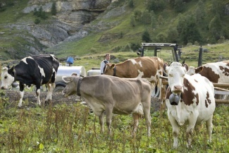
# Visualize 4 images
fig, ax = plt.subplots(2,2, figsize=(8, 8))
for i in range(4):
ax_ = ax[i // 2, i % 2]
ax_.imshow(ds_cow[i].images.numpy())
ax_.axis(False)
fig.subplots_adjust(wspace=None, hspace=None)
fig.savefig("sample_cows.jpg")
 |
 |
 |
 |
When we fine-tune a model, we can change some of its structure. In particular, we will revise the number of classes predicted. Instead of 91 possible options, we will restrict it to only cows and differentiate cows from the background. To change this, we will modify the heads of the model but not the core of the network, where all the object detection information is stored. The core of the network will change as part of the new training process.
Let’s go ahead and run some iterations:
black_box_finetuned = DetectorBox()

black_box_finetuned.train('cows_dataset', epochs=1000)
After running a few iterations (1000) of our model, we can re-check our test images and see how we are doing.
 |
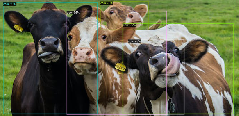 |
It looks better, but does it? We can check! Let’s verify that the metric improved. The new mAP = 0.2316. This is almost double our previous value. Cowincidence? We don’t think so!
Cow-tracking
So far, we have detected individual cows within an image. That’s cool, but we can do better. What if we track individual cows as they move in a video?
The main idea behind object tracking is to do object detection frame by frame (remember that videos are a sequence of images) and then map objects in one frame to the next. One way is to calculate the object’s trajectory and predict where it should be in the next frame. Although this sounds simple, it involves some complex mathematical concepts. But don’t despair. To ease developers’ lives, Tryolabs launched an open-source tool called Norfair that handles all these complexities. And it only takes a few lines of code to get it working!
Take time to read the code in the following cell and unravel what it does:
def euclidean_distance(detection, tracked_object):

"""

The metric that we want to use between consecutive frames

"""

return np.linalg.norm(detection.points - tracked_object.estimate)

black_box = DetectionBox()

video = Video(input_path="cows_running_1.mp4") # path to the original video

tracker = Tracker(distance_function=euclidean_distance, distance_threshold=20)

for frame in video:

detections = black_box.predict(cv2.cvtColor(frame, cv2.COLOR_BGR2RGB))

# Wrap Detectron2 detections in Norfair's Detection objects

dets = [

Detection(p)

for p, c in zip(

detections["instances"].pred_boxes.get_centers().cpu().numpy(),

detections["instances"].pred_classes,

)

]

tracked_objects = tracker.update(detections=dets)

draw_tracked_objects(frame, tracked_objects)

video.write(frame)
Let’s see how Norfair works on a happy cows video:
That looks ok. But, some of the cows get different numbers throughout the video, which means that the tracker cannot correctly recognize them as the same cow. Let’s try to do it with the fine-tuned version.
Can you notice that the marker changes when the cows change direction abruptly? That is related to how the tracking algorithm works! Understanding why the problem occurs will help us find a solution in the next iteration. Remember, training a machine learning model is always an iterative process.
Delving deeper into DetectionBox
By now, you might be wondering: how does the DetectionBox work? And you are right. We have actively ignored that subject so far. We did that because we genuinely believe that the methodological approach to object detection is independent of the model used. We will likely update our default models in a few days, weeks, and months because ML moves fast. Two prominent families of models are used for object detection: YOLOs and RCNNs. In this mini-project, we decided to use Faster-RCNN pre-trained on a ResNet-50 using the CoCo dataset. Do you wanna see a full layer-by-layer explanation of how this deep neural network works? Lucky you asked because we have written a blog post entirely dedicated to answering that question. You should check it out.
Wrapping up
We are approaching the end of this four posts series, which we have enjoyed immensely. What we put in these posts is just the tip of the iceberg. Plenty of other sub-fields, techniques, and resources exist in this vast world of machine learning. We genuinely hope these posts kickstarted your career or interests in machine learning. As we said in our first blog post of the series, we are fans of “learning by doing. ” We encourage you to use the tools you just acquired to go and find new challenges and keep learning.
Finally, remember to inspect some of your predictions manually every time. Otherwise, you will end up with mutant cows.
Diego Kiedanski
AI Solutions Architect, Tryolabs
Germán Hoffman
Engineering Manager, Tryolabs