This blog post was originally published at Tenyks’ website. It is reprinted here with the permission of Tenyks.
We introduce the Multiclass Confusion Matrix for Object Detection, a table that can help you perform failure analysis identifying otherwise unnoticeable errors, such as edge cases or non-representative issues in your data.
In this article we introduce a practical error prediction matrix: the Multiclass Confusion Matrix for Object Detection (MCM). This matrix serves as a good first step to systematically conduct failure analysis of your models.
We describe what the matrix is, and how it allows you to get deeper insights into mispredicted examples. This more granular view of errors can reveal patterns that might go undetected when simply aggregating errors into false positives and false negatives.
We build on our previous article, and use the same example of helmet detection, as shown in Figure 1.

Figure 1. Use-case: detecting classic and welding helmets
Failure analysis in object detection

In a nutshell, failure analysis focuses on examining why an object detector fails on certain inputs, analyzing the causes of the model’s errors or mistakes [1], [2].
At a high level, failure analysis may involve:
- Identifying instances that the model fails on (i.e. incorrect predictions).
- Determining why the model failed on these particular instances (e.g. failing on edge cases the model wasn’t trained on).
- Collecting additional data to address the causes (e.g. gathering more diverse data for the underrepresented categories).
- (Possibly) Improving the model setup (e.g. using a more powerful architecture).
Some of the most common reasons for model failures include:
- Lack of representative training data: The training dataset does not have enough examples of certain objects or scenarios, causing the model to not generalize well.
- Class imbalance: The distribution of the classes in the data is skewed, as a result the model doesn’t learn some classes well.
- Quality of images: The images are degraded by noise, poor lighting, occlusion, or other factors, making the objects difficult to detect.
- Similarity of objects: In this case the model is unable to reliably distinguish between objects that are very similar in appearance.

Figure 2. Bounding boxes affected by occlusion and blur can cause models to fail
Metrics in Object Detection
As we described in our previous post, the primary metric to evaluate object detection performance is mean average precision (mAP). However, when using mAP, failures in object detection can only be coarsely described as false positives or false negatives.
Remember, there are 3 types of predictions in object detection:
- True Positive (TP): correct model prediction. An annotation is correctly matched with a prediction.
- False Positive (FP): incorrect model prediction. The model predicted a bounding box but no corresponding annotation existed.
- False Negative (FN): missing prediction. An annotation is not matched to any prediction (i.e. the object is present but was not detected by the model).
Why grouping together TPs, FPs and FNs is limiting
The downside of organizing predictions in the traditional way (see Figure 3) is that you are left with a numeric score that doesn’t provide any insights to identify why some samples were classified as false positives or false negatives.
Without this information, how can you improve your dataset to have a better model?
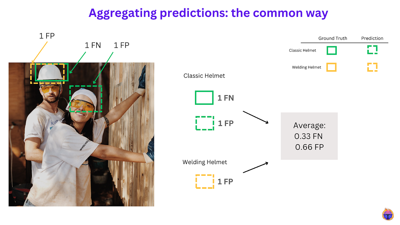
Figure 3. Classic approach to account for false positive and false negative predictions
What if you are tasked to answer questions such as:
- How many examples of Class A did the model confuse with Class B?
- How many undetected predictions were there (e.g. due to non-representative or rare samples)?
- How many examples don’t have any corresponding annotation (i.e. ghost predictions)?
A solid first step to answering the previous set of questions is to use the Multiclass Confusion Matrix for Object Detection (MCM), which is described below.
Multiclass Confusion Matrix for Object Detection
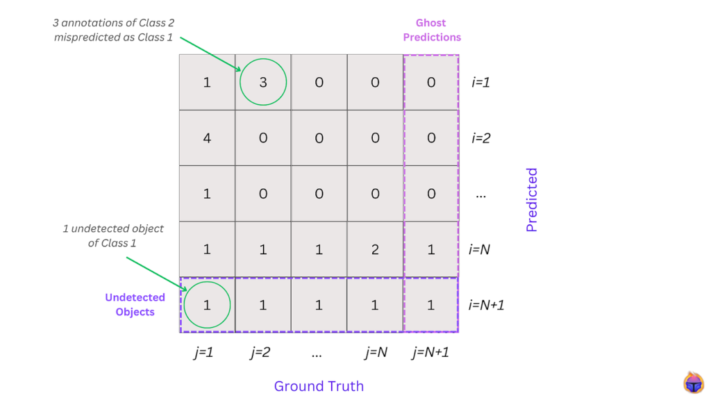
The MCM arranges predictions into an (N+1) * (N+1) matrix (where N is the number of classes). Every cell (i, j) specifies the number of matched bounding boxes that were predicted as class i (or not predicted, if i=N+1), and had an annotation class j (or no annotation, if j=N+1).
Selecting the best match across all classes, not just within the same class
Given a ground truth label, this matrix finds the best matching prediction, even if the predicted label is from a different class than the true label.
For example, in our helmet detection task, this matrix might select a “classic helmet” prediction as the best match for a true “welding helmet” label, if this is a better option. This allows the MCM to capture errors where the model confuses one class for another, rather than just errors within the same class.

Figure 4. The Multiclass Confusion Matrix for Object Detection
This closely resembles multiclass confusion matrices used in classification, with the addition of “Undetected” and “Ghost Prediction” rows and columns.
In particular, the MCM defines 4 types of predictions:
- True Positive: correct model prediction. A prediction is matched with an annotation of the same class (this definition is the same as always).
- Undetected: missing model prediction. An annotation is not matched to any prediction (this definition is the same as the False Negative definition from before).

- Mispredicted: incorrectly-predicted class. A prediction is matched with an annotation of a different class (this would have been graded as a False Positive).

- Ghost Prediction: incorrect prediction. A prediction is not matched with any annotation (this would have also been graded as a False Positive).

How can the MCM improve your failure analysis process?
The MCM offers a more granular view into your model errors, including:
- Observing how errors are distributed across class combinations (instead of producing a single aggregate score, such as mAP, or AP)
- Better understanding the different types of errors (i.e. is it a ghost prediction, misprediction, or undetected case?)
This type of analysis can be invaluable in gaining a deeper understanding into why & where your model is failing. For instance:
- A high number of mispredictions between two classes can indicate a poor class definition, in which both classes share a lot of common samples. For instance, if you have classes “Pedestrian” and “Cyclist”, but then you have many samples of a person walking next to a bike.
- A high number of undetected objects could mean a large number of outliers and edge cases (i.e. data representativity issues). For example, cars of an unusual color, or old models of cars that are not frequently-present in the dataset.
- A high number of ghost predictions could indicate the need to set a higher confidence threshold for the model, or could indicate a low representativity of certain cases in your data. For instance, if you have a small number of cyclist samples, your model may start to incorrectly detect parked bikes as cyclists.
This kind of analysis is impossible to conduct on aggregate metrics, such as mAP or mAR.
In comparison to aggregating predictions into FP, and FN, Figure 5 shows a MCM table, where the predictions lie on the Y axis, and the ground truth labels are on the X axis:
- The misprediction occurs because for a classic helmet ground truth label (green solid bounding box on the left side), the model predicts a welding helmet (yellow dashed bounding box).
- The ghost prediction takes place because the model predicts a classic helmet (green dashed bounding box in the center) but this object does not exist in our ground truth labels.
Key takeaway: The Multiclass Confusion Matrix for Object Detection (MCM) helps you identify undetected objects, ghost predictions, and mispredictions in a more intuitive way than simply using TP, FP, and FN.

Figure 5. The MCM helps you quickly spot undetected, ghost predictions and mispredicted instances
Example: Identifying undetected pedestrians in the Kitti dataset
In this section we provide a practical application example of the Multiclass Confusion Matrix for Object Detection (MCM), using the Tenyks platform.
Kitti dataset: We use Kitti, a popular dataset containing data for object detection, tracking, depth perception, and more — all from real-world driving scenarios. This makes it useful for machine learning models in self-driving cars, where not detecting pedestrians 🚶 is very dangerous, since disastrous consequences can happen when a self-driving car fails to spot a pedestrian in time.
Figure 6 shows how the MCM helps you quickly visualize where a trained detector fails at detecting pedestrians: after clicking on the number of undetected objects with the ground truth label of Pedestrian, you can see what images contain these undetected samples.
Beyond that, using the Tenyks platform you can filter out these undetected objects to obtain more insights into why the model failed to predict these examples. As Figure 6 shows, many of the undetected Pedestrians objects are occluded, noisy or are very small. This is a truly effective way of investigating the root cause of why your model is failing, which is the first step to devising a strategy to improving your model’s performance!
Figure 6. The Multiclass Confusion Matrix for Object Detection (MCM) in action!
Summary
In this post we introduced the Multiclass Confusion Matrix for Object Detection (MCM), a granular first step to help you identify model failures in object detection. This matrix categorizes predictions into true positives, undetected, mispredicted and ghost predictions. The MCM allows you to identify samples that may lead to problems in your dataset such as edge cases or representative issues, that otherwise would go unnoticed by traditional approaches.
The road ahead: a hierarchical approach!
Generally, we can breakdown error analysis of an object detection model into three scenarios:
- High-level error analysis: including aggregate metrics such as mAP, mAR, TP, FP, and FN.
- Medium-level error analysis: a more granular approach than the previous one, such instance MCM.
- Low-level error analysis: a very low-level, detailed view of what is wrong and why, conducted by automatic strategies such as Data Quality Checks.
The Tenyks platform enables analysis of failure cases at all three different levels. As we have covered in this Series, you can analyze errors at the high and at the medium level. In the upcoming third instalment, we will explore how Tenyks enables Data Quality Checks to identify systemic issues, at the very low-level, that may be impacting model performance.
By examining failures at these three hierarchy levels, you can gain a holistic understanding of the weaknesses in your model and data, and take targeted actions to improve results.
Stay tuned!
Note: All images for this post are from unsplash.com based on the unsplash license.
References
- Why Object Detectors Fail: Investigating the Influence of the Dataset
- Imbalance Problems in Object Detection: A Review
Authors: Jose Gabriel Islas Montero, Dmitry Kazhdan.