In this dynamic technology landscape, the fusion of artificial intelligence and edge computing is revolutionizing real-time data processing. Embedded vision and edge AI take center stage, offering unparalleled potential for precision and efficiency at the edge. However, the challenge lies in executing vision tasks on resource-limited edge devices. Model compression techniques, notably quantization, emerge as crucial solutions to address this complexity, optimizing computational power and memory usage.
In this series of articles, we will explore the critical concepts of compression, focusing first on quantization as an essential strategy for optimizing vision tasks on the edge. We will delve into how these techniques can help address the constraints of edge computing and make vision applications feasible and efficient in these environments.
Embedded Vision and Edge AI Applications
Let’s delve deeper into the promising areas of deploying vision-based tasks on the edge and explore the wide range of applications that benefit from this transformative technology:
- Surveillance: On-device vision processing enhances security by analyzing live video feeds, detecting anomalies and triggering real-time alerts.
- Autonomous Vehicles: Edge devices on self-driving cars process data locally, ensuring rapid decision-making for navigation, object detection, and collision avoidance even in low-connectivity areas.
- Virtual/Augmented Reality (VR/AR): Edge AI is essential for superior real-time performance, enhanced power efficiency and a compact form factor in VR/AR applications.
- Industrial Automation: Edge-based vision in manufacturing facilitates real-time monitoring, defect inspection and quality control, reducing downtime and enhancing security.
- Healthcare and Telemedicine: Edge AI optimises medical imaging for rapid on-site assessments and provides real-time visual data for virtual consultations, improving immediate guidance and support.
Model Compression Techniques
Model compression techniques are crucial for edge computing, reducing deep learning model size for lower memory and processing needs. Key techniques include:
- Knowledge Distillation: A large model (teacher) trains a smaller one (student), maintaining accuracy on edge devices with reduced weight.
- Pruning/Sparsity: Removing unimportant weights creates a smaller, faster-executing model.
- Quantization: Reducing numerical precision, such as converting from 32-bit to 8-bit values, significantly cuts memory and computation costs, though it may impact accuracy.
- Efficient Architectures: Models like MobileNet and SqueezeNet are designed for edge computing, offering compactness and computational efficiency without sacrificing performance.
Implementing these techniques tailors models for edge computing, enabling real-time processing on resource-constrained devices for applications like IoT, autonomous vehicles, and augmented reality.
Quantization
Quantization is vital in edge AI, converting high-precision floating-point numbers to fixed-point or integers. This reduces memory demands, enabling efficient processing on resource-constrained devices while maintaining acceptable accuracy. Traditional AI models with 32-bit or 64-bit floating-point numbers face significant burdens. Quantization, often to 8-bit integers, substantially reduces the model’s footprint and processing time, fitting comfortably within edge device constraints. Despite accuracy concerns, modern quantization minimizes impact through strategic bit allocation. However, achieving the right balance remains a nuanced challenge. This section will delve into key considerations like conversion equations, quantization schemes, bit width, min/max tuning, and quantized operations.
Quantization Scheme
Quantization is the process of mapping real numbers, denoted as ‘r’, to quantized integers, represented as ‘q,’ and is expressed by Equation 1. Here, ‘S’ and ‘Z’ are the scale and zero-point quantization parameters, respectively. For an N-bit quantization, ‘q’ is an N-bit integer, ‘S’ typically takes on a floating-point value, which is represented using fixed-point notation, and ‘Z’ is of the same data type as the quantized value. An important constraint on the zero-point is imposed to ensure that real zero values are quantized without any error. The quantized values can be converted back to real values using Equation 2.
q = round (r/S + Z)
Equation 1. Quantization
r = S(q – Z)
Equation 2. Dequantization
Now, let’s delve into how the quantization parameters ‘S’ and ‘Z’ can be determined in cases where the real-world data is floating-point in distribution. These parameters are influenced by the range of real values as expressed in Equations 3 and 4, where r_max/min stands for the range of float point values and q_max/min is the range of quantized values.
S = (r_max – r_min) / (q_max – q_min)
Equation 3. Scale Calculation
Z = round (q_max – r_max / S)
Equation 4. Zero-point Calculation
When data is quantized, there is an inherent loss of information, leading to discrepancies between the original data and the quantized representation. These discrepancies result in what is known as quantization noise. The severity depends on parameters like scale/offset and bit depth. Quantization noise could potentially impact the accuracy of the model’s predictions. Striking a balance between model compression through quantization and minimizing the adverse effects of quantization noise is a key challenge in making AI models efficient.
Based on the data distribution, to minimize quantization error, the best choice of quantization falls into two broad categories:
Quantization Types
Symmetric Quantization
This implementation assumes the quantization is symmetric around zero as shown in Figure 1, which allows the quantization parameter zero-point Z = 0. This allows for efficient implementation of integer arithmetic by eliminating the handling of zero-point.
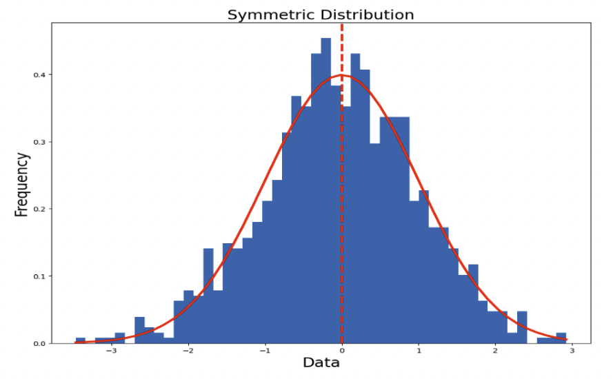 Figure 1. A symmetric distribution with zero point = 0
Asymmetric Quantization
Asymmetric quantization, shown in Figure 2, optimizes efficiency by adjusting the scale and zero point to align with the distribution of the quantized data. This minimizes quantization error, albeit with an increase in computational overhead.
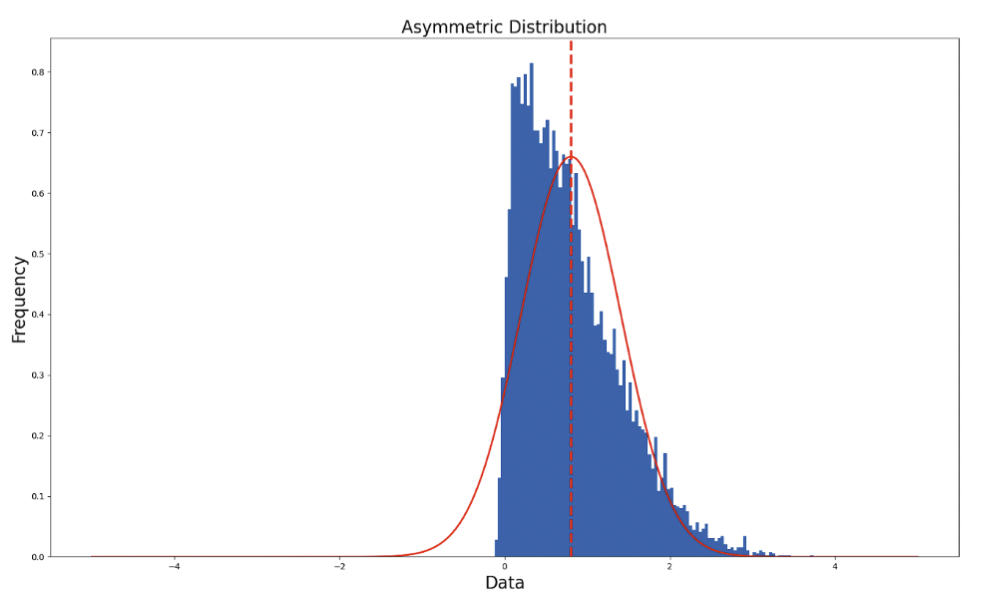 Figure 2. An asymmetric distribution with non-zero zero point
Choosing between symmetric and asymmetric quantization hinges on balancing accuracy and performance. Symmetric quantization, without a zero point, enhances efficiency in operations like matrix multiplication or convolutions. Asymmetric quantization prioritizes accuracy by offering enhanced precision where it matters most, minimizing errors in data-concentrated regions. The decision relies on a thorough understanding of data distribution, tailored to the application and target device requirements.
Figure 3 shows how asymmetric quantization can be used to handle shifts in the data distribution, while symmetric distribution might lead to excessive quantization noise due to its inability to quantize resolution effectively.
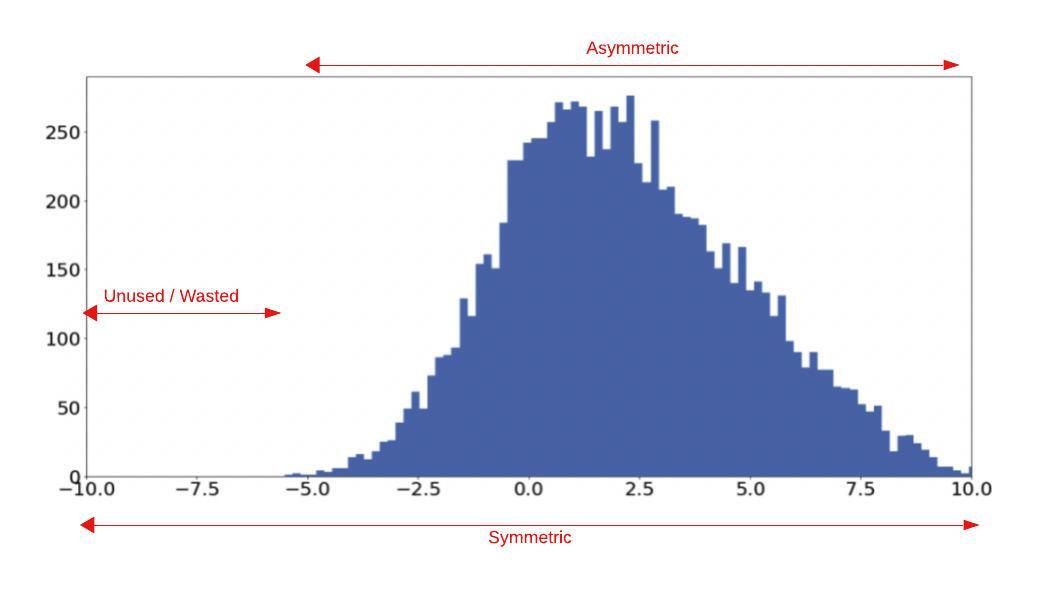 Figure 3. The effects of scale and shift parameters in symmetric and asymmetric quantization
Quantization Resolution
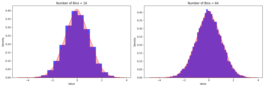
In data quantization, the number of bits (N) is critical, impacting precision and resource needs. Fewer bits reduce precision but increase quantization error, risking information and accuracy loss. More bits enhance precision but require higher resources, crucial in edge computing with limited resources. Balancing bits and precision is vital in applications like embedded vision and edge AI, where insufficient bits may compromise accuracy but excess bits strain resources. Data scientists and engineers must meticulously assess the unique requirements of their intended application. Figure 4 shows the float distribution and its quantized results for different N-bit quantization. The error is significantly reduced for larger N-bit quantization. The figure shows the effects of quantization for different quantization levels, i.e., 16 levels for N = 4 and 64 levels for N = 6, respectively. In a real-world application, these quantization levels are decided based on the number of bits used for quantization.
 Figure 4. The effect of quantization levels on quantization noise
Range Tuning (Min/Max Parameters)
Selecting min/max values for quantization, known as dynamic range scaling, is crucial for optimizing data processing, especially in limited precision scenarios. This choice impacts the balance between precision and efficiency. The right range ensures an appropriate dynamic span, preserving essential information while reducing quantization noise. Too narrow a range may cause data clipping and information loss, while too wide a range may inefficiently use quantization levels, increasing noise. Data scientists use dataset statistics to determine suitable min/max values, capturing data variability while optimizing resource usage.
When quantizing deep learning models, these min/max values are calibrated using a representative dataset, ensuring precision for relevant data and preventing outliers. Weight ranges are fixed in trained models, presenting opportunities for efficient quantization. Activation distribution, dependent on network input, is estimated using the range stored during training or a calibration dataset for quantization.
Mean/Standard Deviation
Mean and standard deviation determine min/max clipping, ideal for distributions approximating a Gaussian shape centered around the mean (Equation 5).
min/max = μ +/- 3σ
Equation 5. Mean and standard deviation determination of min/max clipping
Histogram
Histogram-based methods use percentiles to select the quantization range, typically large enough to be representative and avoid outliers that might impact accuracy. The range is set based on the distribution of absolute values during calibration. For example, a 99% calibration clips 1% of the largest magnitude values, efficiently eliminating potential outliers.
Moving Average
The default implementation of TensorFlow uses moving average to update the min/max values for each iteration of the calibration dataset.
Entropy
Min/max values minimize distribution entropy using KL divergence, reducing information loss between original floating-point values and the quantized format. This is TensorRT’s default method, especially valuable when tensor values to be quantized are equally important.
More to Come
In our next article, we will embark on a journey into the realm of convolutional neural networks (CNNs), with a focus on how these quantization schemes are applied, a crucial process in optimizing these powerful models. Stay tuned as we unveil compelling results derived from diverse quantization schemes, shedding light on the transformative impact these techniques have on the landscape of deep learning.
Dwith Chenna
Senior Computer Vision Engineer, Magic Leap