This blog post was originally published at Digica’s website. It is reprinted here with the permission of Digica.
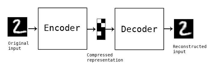
Autoencoders have existed in Data Science for a long time. This type of model has three sequential parts: the input layer (encoder); the hidden layer; and the output layer (decoder). It seems like a simple concept, but it is very powerful. You use autoencoders as an unsupervised method, which means that labels are not used in their training process.
[https://blog.keras.io/building-autoencoders-in-keras.html]
Autoencoders can reconstruct original input from a compressed representation known as a hidden layer or latent space. Autoencoders can also be used on compressed data. Compressed data can be especially useful if the dataset is large, and therefore difficult to fit into the available computer memory. Compared to other compression algorithms, autoencoders are dedicated only to the data on which the model was trained. This means that if the autoencoder was trained on images, it cannot be used on, for example, audio files. For another type of data or different dataset, you must train a new autoencoder.

A very similar application is for the purposes of dimensional reduction. One of the problems in machine learning is how to deal with a large number of data dimensions or features, a problem which is sometimes called the “curse of dimensionality”. Usually, data with a very large number of features or dimensions is also sparse. Sparse data is problematic because every sample is far from the next sample in hyperdimensional space. If samples are lying far from each other, it is difficult to carry out clustering based on either distance or on classification using the K-Nearest Neighbours algorithm or a Support Vector Machine. In addition, reducing the number of features, or the size of images, enables easier visualisation of the dataset. This makes it easier to understand the relationships hidden in the data, and to see the variations across the data.
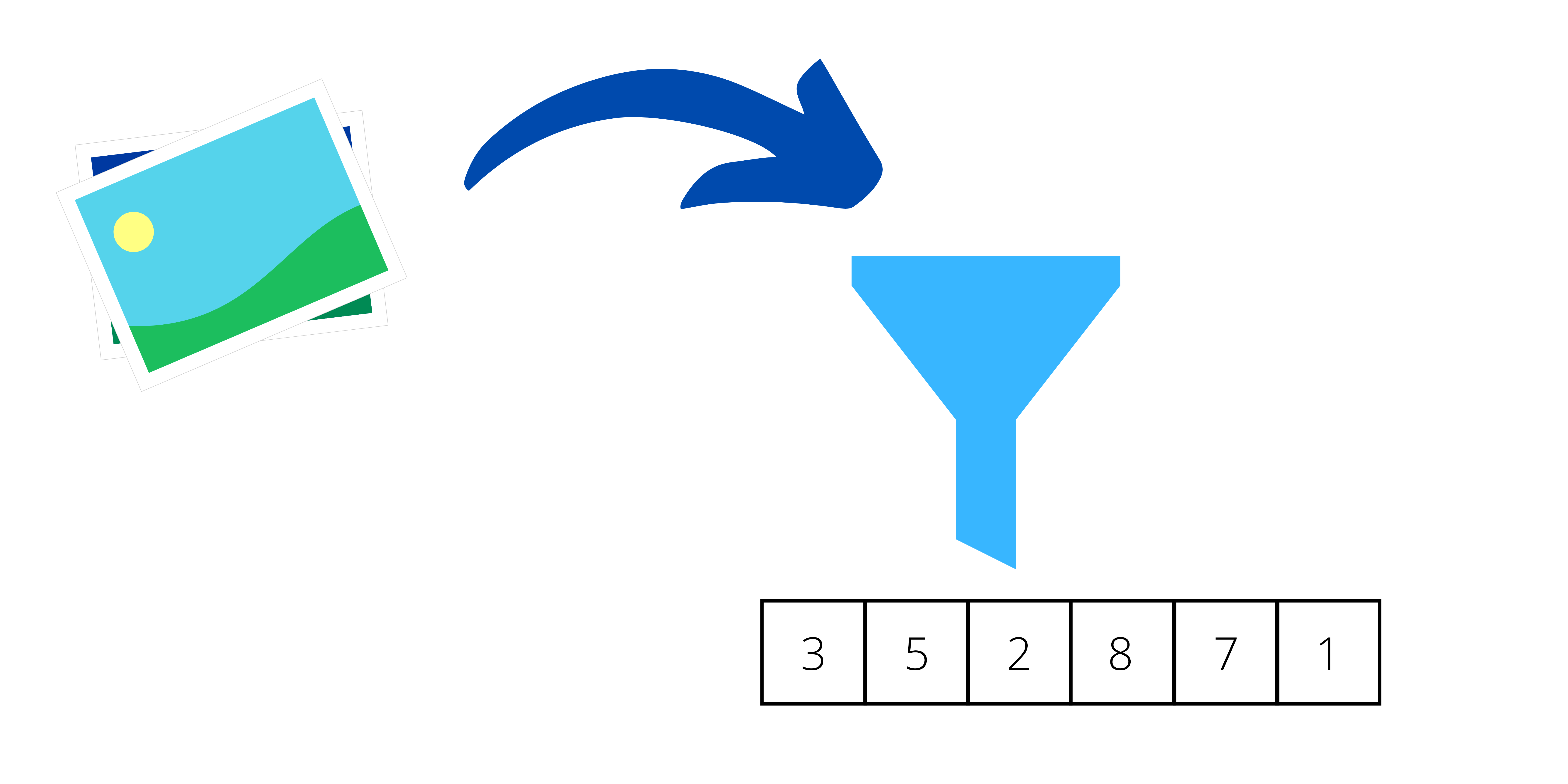
Compressed representation (also known as latent space) is one of my favourite things in autoencoders because it can be used as a tool for engineering features. Sometimes Data Scientists spend a lot of time coming up with ideas for new features. The simplest way is to calculate some statistical values, for example, average, median, standard deviation, and so on. On the other hand, if you have domain knowledge, you can measure certain parameters, and then add or create useful features. Processing all this data and creating new features is time-consuming. And sometimes it is difficult to come up with an idea for a feature that leads to differentiating between objects in the domain. Fortunately, latent space can be used for this purpose.
Autoencoders create the most meaningful features in a given context.
In a predefined size of latent space (predefining is done when preparing the architecture of the model), the most meaningful features must be present. This is because, from this small piece of information, the original input should be recreated as well as possible. So, thanks to that, you have “a thick, meaty soup” of information there. The only problem is that those features cannot be interpreted by humans. For example, if you put an image of a cat into an autoencoder, you cannot say that feature A in latent space represents “triangular ears”, that feature B represents “a long tail with fur”, and so on. But, if you do not need to fully understand each feature in your model, you should seriously consider using the latent space in your classifier.
Another thing which I like about autoencoders is that one of their types can reduce noise in the data. For image data, Gaussian or median filters are frequently used to reduce noise. But another way of removing noise is to use autoencoders. You may be wondering why noise can be reduced by autoencoders when they are designed to recreate an original image as well as possible. The reason why they can do this lies in the nature of latent space itself. As I wrote above, latent space contains the most meaningful features of the input data. If all the input data has noise, the noise seems like useless information. And because it is redundant information in relation to the image, no feature in latent space retains information about the noise.
When working as a Data Scientist, I work not only on clustering and classification tasks, but also on the task of detecting anomalies, which means identifying that a given sample falls outside the bounds of the rest of the data. Of course, you can treat this as yet another classification task, but this approach is more difficult because of the imbalance in the dataset (the ratio of one class to another class is much higher than 1:1). Alternatively, you can use algorithms that are dedicated to solving this problem by using, for example, the Isolation Forest algorithm or the One-Class SVM algorithm. However, you can also use autoencoders to detect anomalies. In this case, the training process is not run on all samples of a given training dataset, but only on “normal” samples in that set, that is, on samples without any anomalies. For the training set, the reconstruction error rate should be as low as possible. This means that the autoencoder has learned how to recreate data from the original input data. Then you use the autoencoder to process data which is different from the original data. In this case, the reconstruction error rate should be relatively high compared to the low error rate for the training set. If you then plotted a histogram of the two reconstruction error rates, you would clearly see that the distribution of reconstruction errors is quite different between the two sets of data. On that basis, you can then set the threshold of the error value which classifies samples as an anomaly.
Most of the examples that I have mentioned above are about data that represents an image. However, you can use whichever type of data that you wish, for example, tabular data, audio files or text data. The architecture of an autoencoder can incorporate convolutional layers, recurrent layers and LSTMs. In basic autoencoder models, there is only one “dense” layer, but your autoencoder can have a number of different layers. When designing the architecture for an autoencoder, the most important thing is to ensure that the encoder part leads to a bottleneck in the second, hidden, layer of the model. After the data has passed through the hidden layer, the sample is then reconstructed from the sets of smaller representations in the third layer, which enlarges latent space to the size of the original sample.
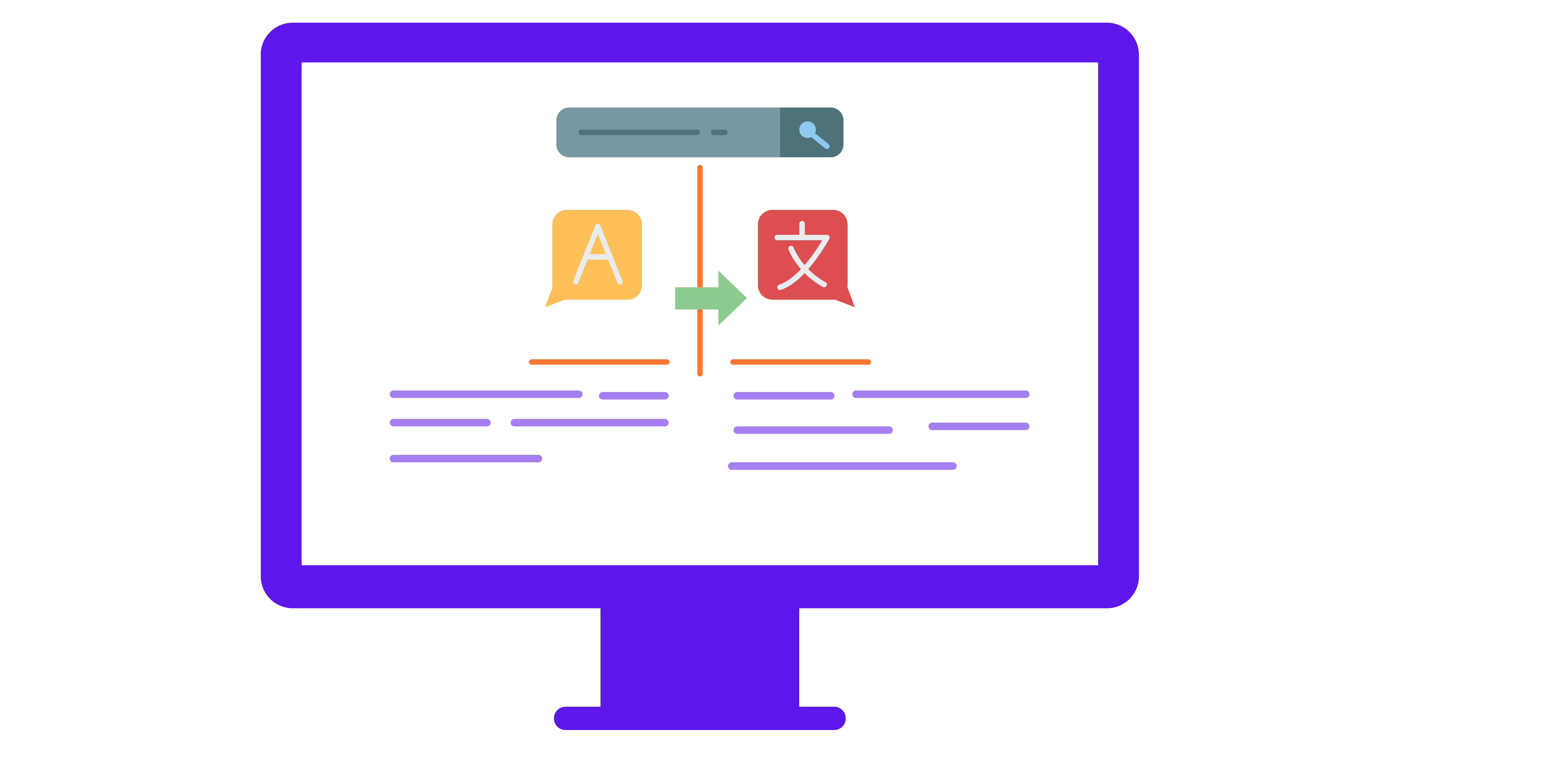
Autoencoders are also used in natural language processing, for example, in machine-translation. In this case, a text that is written in one language is processed into a compressed representation which stores the “meaning”, and from that it is possible to recreate the same message in other languages. In the same way as described in the paragraph above, when it comes to machine-translation, latent space contains the most meaningful information extracted by the encoder.
As you can see from all the different examples in my article, autoencoders have many usages in data science. I have mentioned compressing data, dimension reduction, feature extraction, noise reduction, anomaly detection and machine translation. These usages all have great potential because they can be used to solve many AI problems and, depending on a given architecture, autoencoders can be used for many different data types, including tabular data, images and texts. What’s more, as an autoencoder is an unsupervised method, there is no need to introduce data labels, so this avoids many technical problems and is almost certainly less costly.
Joanna Piwko
Data Scientist, Digica