Enable Pose Detection on Snapdragon X Elite: Step-by-step Tutorial

This article was originally published at Qualcomm’s website. It is reprinted here with the permission of Qualcomm.

I know why you’re here; you’ve decided to buy your first device with Snapdragon X Elite processor, awesome choice! You now ventured over to Qualcomm AI Hub, grabbed a model and excitedly watched as it downloaded.

“Hmmm okay… now what?”

You click the Model Repository link hoping for next steps. It does tell you something but also nothing at all.

Luckily, you no longer have to guess or figure out the next steps. By the end of this walkthrough, you will have a clear step-by-step understanding of how to get from downloading the model to inference and beyond.

Although we’ll be using HRNetPose for this walkthrough, the process should apply to most models currently available on Qualcomm AI Hub (LLMs are coming!).

As a bonus, you’ll also leave with a basic understanding of how to utilize ONNX Runtime for inference.

So, grab your brand-new Snapdragon X Elite and let’s make it happen!

Overview

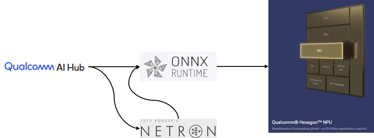
The goal of this guide is to walk you, the developer, through all the necessary steps to run a model using Qualcomm Hexagon NPU, without the need to dig through endless docs possibly losing your sanity, or even worse your motivation, in the process.

The HRNetPose Detection Application will be built in Python, using tools like Qualcomm AI Hub, onnxruntime-qnn, Jupyter Notebook, OpenCV, and NumPy.

By the end of this walkthrough, you will have a fully working application that runs on Hexagon and detects 17 body keypoints using the HRNetPose model. This guide will create the bridge between “I downloaded a model!” and “I actually did something!! Now I’m ready to take over the world!”

Preparation

Let’s get the entire development environment set up, we will assume that you have a completely new laptop with Snapdragon X Elite. Some requirements may be skipped if you’re already a Snapdragon X Elite veteran.

Requirements:

1. Visual Studio Installer
   1. Workloads – Desktop development with C++
   2. Components – MSVC v143 – VS 2022 C++ 64-bit build tools (latest)
2. Python 3.11.0
   1. Windows installer (ARM64)
      1. https://www.python.org/ftp/python/3.11.0/python-3.11.0-arm64.exe
3.  HRNetPose Model (quantized version)
   1. Download from Qualcomm AI Hub
      1. https://aihub.qualcomm.com/compute/models/hrnet_pose_quantized?domain=Computer+Vision&useCase=Pose+Estimation
4.  Python Packages
   1. virtualenv
   2. OpenCV – Windows on Snapdragong not yet supported
      1. https://github.com/DerrickJ1612/qnn_arm64_wheels/tree/main
   3. Onnxruntime-qnn
   4. Pillow
5. Jupyter Notebook

Setup:

Let us now set the stage. First, we need to download and install Visual Studio Installer and Python 3.11 ARM64, we’ll currently use a strict version of python-3.11.0-arm64. Why? Because we may need to use an OpenCV wheel that was built from source using this exact environment, hopefully we don’t but if we do, we’ll be ready!

Once we have the correct Python version installed the necessary workloads and components from Visual Studio Installer, we’ll load PowerShell and ensure that we’re seeing the correct Python version using the command below.

Windows makes it convenient to check and use a specific Python version using the py command, this is especially useful if you’re juggling multiple Python installs on your system.

>> py -0
 Output << -V:3.11 * Python 3.1 (64-bit) >>

We’ve now verified that we have the correct Python version, so let’s create a world inside of a world aka our virtual environment.

I highly recommend using a virtual environment. It keeps your dependencies in check and your development setup clean, organized, and isolated from all the chaos that always finds its way into your global Python install.

First, we need to install the virtualenv module, which we’ll use to create our environment.

>> py -V 3.11_arm64 -m pip install virtualenv

Next, we’ll create our virtual environment

>> py -V 3.11_arm64 -m virtualenv env_hrnetpose

Let’s activate the virtual environment we just created and make sure we are using the correct Python version.

>> env_hrnet_pose/Scripts/activate.ps1
>> python -c “import platform;print(platform.machine()); print(platform.processor())”

If you’re seeing AMD64, you’ve likely downloaded the wrong Python version.

We’ll begin installation of OpenCV, onnxruntime-qnn, pillow, and notebook Python packages.

At the time of this walkthrough, OpenCV does not have official pre-built wheels for Windows on Snapdragon. Before diving into more painful territory, let’s take a moment, cross our fingers, and hope that all the stars have aligned and Windows on Snapdragon is now supported.

>> pip install opencv-python

If support is still non-existent, Plan B

>> pip install opencv-python-aarch64

Still nothing?!?! Deep breath. Time to get a little more involved.

First, clone the repo in step 4b of Requirements (listed in the beginning of this article), then run

>> pip install opencv/opencv-4.11-py3-none-any.whl

If you make it this far and things still aren’t working, please head over to our Discord server and make some noise. Vent, kick – we get it. This should be way easier!

And if you’re feeling brave and fearless, another option is to clone OpenCV and build from source. It works, I promise, but only as a very last resort. You can also go to our Discord server if you’d like help going down this rabbit hole, our Discord is your friend. But really, you should never have to go down this path.

Let’s continue with less painful installs:

>> pip install onnxruntime-qnn
>> pip install pillow
>> pip install notebook

Of course, you could also have run the command below and got everything in one shot.

>> pip install -r requirements.txt

Building and Running App

Time for a quick (and optional) commercial break.

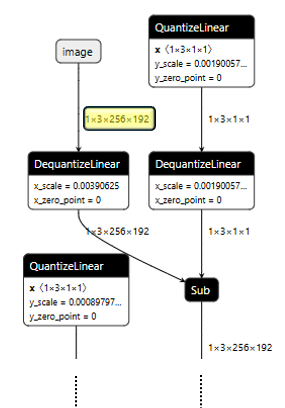
Let me introduce you to Netron, a viewer for neural network models that let you visualize layers, tensor shapes, and connections.

We’ll use Netron to peek inside the HRNetPose model we downloaded from Qualcomm AI Hub. This step isn’t required, but I like to nerd out and explore the model’s structure as well as get a visual sense of the expected inputs and outputs before diving into code.

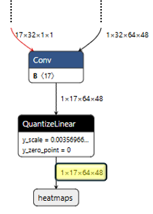
The images below are directly from Netron, the highlighted fields show the expected model input and output.

After model inspection we’re now ready for the fun part, let’s start coding.

The first thing we should do is ensure that we are in the correct Python environment…… again!

import platform

arch = platform.machine()
sys = platform.system()
processor = platform.processor()
print(f"{arch}\n{sys}\n{processor}")

As with any great adventure we need to make sure we have the appropriate gear before starting, i.e. imports.

Obviously, we’ll need onnxruntime specifically the onnxruntime-qnn backend to run inference on Hexagon.

Then there’s OpenCV (cv2), which may or may not throw an annoying recursion error just to keep things interesting. I’m still root-causing this because of course, “iT wOrKs On My CoMpUtEr.”

This error may or may not pop up when trying to import cv2 and will only occur if you resorted to cloning the wheel repo and pip install from that repo.

Lastly, we’ll need NumPy, and just a few other imports to help us with image processing and path handling.

import os

import onnxruntime as ort
import cv2 as cv
improt numpy as np

from PIL import Image
from pathlib import Path

Let us now setup all the necessary paths so that we don’t have to keep typing this over, and over, and over, and over again.

We’ll first grab the root directory of this notebook we also need to dynamically find root directory to onnxruntime. This is important because when we pip install onnxruntime-qnn, it conveniently includes the Hexagon drivers that we need to pass to our InferenceSession.

What this also means is:

• No need to search Qualcomm’s website.
• No SDK scavenger hunting.
• No figuring out what a Nuget even is.

Just a quick pip install, and we’re ready to roll!

TL;DR this path gives us access to important things.

We then point to our model, which also gets passed to the InferenceSession.

# Path to notebook root directory
root_dir = Path.cwd().parent

# Path to onnxruntime root directory within our virtual environment
onnxruntime_dir = Path(ort.__file__).parent

# Model location
model_subdirectory = "hrnet_pose"
model_name = "hrnet_quantized.onnx"
model_path = Path.joinpath(root_dir,"models",model_subdirectory,model_name) 

# Location of Hexagon driver
hexagon_driver = Path.joinpath(onnxruntime_dir,"capi","QnnHtp.dll")

With all the paths set up, we can now easily and cleanly initialize our inference session.

Since we want to use the QNNExecutionProvider, we’ll need to point the inference session to the Hexagon driver. If the Hexagon driver path isn’t available (or is incorrect), ONNX Runtime will fall back to running on CPU using the CPUExecutionProvider.

We also add the path to our model when initializing the session.

qnn_provider_options = {
    "backend_path": hexagon_driver,
}

# Creating the onnxruntime inference session
session = ort.InferenceSession(model_path, 
                               providers= [("QNNExecutionProvider",qnn_provider_options),"CPUExecutionProvider"],
                              )

## Retrieve expected input from model
inputs = session.get_inputs()
outputs = session.get_outputs()
input_0 = inputs[0] 
output_0 = outputs[0]
session.get_providers()

The output from session.get_providers() should be:

['QNNExecutionProvider', 'CPUExecutionProvider']

If you used Netron, then you already have an idea of what the model inputs and outputs are. We can also get this information directly from the session.

Let’s do a few sanity checks to understand what inputs the model expects. This will help guide our image pre-processing steps.

print(f"Expected Input Shape: {input_0.shape}")
print(f"Expected Input Type: {input_0.type}")
print(f"Expected Input Name: {input_0.name}")

Output>>>

Expected Input Shape: [1, 3, 256, 192]
Expected Input Type: tensor(float)
Expected Input Name: image

We’ll now check what comes out of the model, so we have an idea of what post-processing steps we need to take.

print(f"Expected Output Shape: {output_0.shape}")
print(f"Expected Output Type: {output_0.type}")
print(f"Expected Output Name: {output_0.name}")

Output>>>

Expected Output Shape: [1, 17, 64, 48]
Expected Output Type: tensor(float)
Expected Output Name: heatmaps

Now that we have our session set up, let’s create a helper function to transform an input image into the format our model expects (1, 3, 256, 192).

The purpose of this function is to take an input, and an expected shape. The function then resizes, type cast, and scale the pixels of the input image.

This function will return a tuple with just our scaled and type casted image as well as another image that we reshape into the format that’s expected by model.

We’ll cover this more later.

expected_shape = input_0.shape

def transform_numpy_opencv(image: np.ndarray, 
                           expected_shape: Tuple[int, int],
                          ) -> Tuple[np.ndarray, np.ndarray]:

    height, width = expected_shape[2], expected_shape[3]
    resized_image = cv.resize(image, (width, height), interpolation=cv.INTER_CUBIC)
    float_image = resized_image.astype(np.float32) / 255.0
    chw_image = np.transpose(float_image, (2,0,1)) # HWC -> CHW

    return (float_image,chw_image)

The last helper function we’ll create handles post-processing the model outputs. It takes in the raw outputs after inference, along with two scaling values one for height and one for width.

Let’s quickly recall the model’s expected output shape from above (1, 17, 64, 48). What exactly does this mean?

• The 1 is the batch size, which we can ignore for this app.
• The 17 is a bit more interesting, I’ll save you time by telling you that it corresponds to the 17 standard human body joints based on the COCO dataset. These key points identify things like nose, ears, knees, ankles, shoulders, etc.
• 64, 48 correspond to the height and width of the heatmaps that are returned from the model.

Altogether, we get 17 different heatmaps, each of shape (64,48). This function will iterate through each heatmap, find the index of the maximum value (i.e point with highest confidence), then convert this index to the corresponding height and width coordinates relative to heatmap.

For example, if the current heatmap corresponds to the left shoulder, the function will find where the maximum value is and provide coordinates of this point, the point is where the model predicts the left shoulder is located within the heatmap.

Once we’ve done that for all 17 heatmaps, we’ll have a full set of predicted keypoints mapped to the original image dimensions.

def keypoint_processor_numpy(post_inference_array: np.ndarray, scaler_height: int, scaler_width: int ) -> List[Tuple[int, int]]:
    keypoint_coordinates = []

    for keypoint in range(post_inference_array.shape[0]):
        heatmap = post_inference_array[keypoint]
        max_val_index = np.argmax(heatmap)
        img_height, img_width = np.unravel_index(max_val_index, heatmap.shape)
        coords = (int(img_height * scaler_height), int(img_width * scaler_width))
        keypoint_coordinates.append(coords)

    return keypoint_coordinates

Let’s put it all together. We’ll start by using OpenCV to initialize our camera. If you pass 0, your Snapdragon X Elite will use the built-in system camera. If you plug in an external webcam, you can pass a 1 to use that instead.

After that we’ll do a quick check to ensure the camera initialized properly:

# 0: System Camera
cap = cv.VideoCapture(0)

if not cap.isOpened():
    print("Invalid Camera Selected")
    exit()

Let us now figure out the scaler that we’ll pass to our keypoint_processor function. Below will automatically grab the expected scalers:

###########################################################################
## This is for scaling purposes ###########################################
###########################################################################
input_image_height, input_image_width = expected_shape[2], expected_shape[3]

heatmap_height, heatmap_width = output_0.shape[2], output_0.shape[3]
scaler_height = input_image_height/heatmap_height
scaler_width = input_image_width/heatmap_width

No secret, the scaler is 4 for both height and width. After going back to the original paper, knowing exactly what I’m looking for, and performing a little quantum physics with a side of multivariate calculus, I discovered (buried somewhere in the depths of academia) the fact that the input images of (256, 192) are scaled down by four to get heatmaps of (64, 48) is actually mentioned in some very obscure way.

Anyway, rant over, back to coding.

Now we’re going to enter our main runtime loop that continuously.

• Capture frames from the webcam
• Performs inference
• Post-process the results
• Displays the frame with keypoints overlaid.

In other words, we’re officially on the home stretch!

Let’s capture our first image using OpenCV and check that we received something valid:

while True:

    ret, hwc_frame = cap.read()
 
    if not ret:
        print("Can't receive frame (stream end?). Exiting...")
        break

Quick Note: The image that we capture has a shape (height, width, channel) which is why I name the variable hwc_frame.

Our model, however, expects an image size of (batch, channel, height, width) ignore batch and lets just focus on (channel, height, width) part.

This is exactly why we use our transform_numpy_opencv() helper function, it reshapes, type casts, and normalizes the image.

while True:

    ret, hwc_frame = cap.read()
 
    if not ret:
        print("Can't receive frame (stream end?). Exiting...")
        break

    hwc_frame_processed, chw_frame = transform_numpy_opencv(hwc_frame, expected_shape)

As mentioned earlier, we now have two frames.

1. Frame 1 is (almost) ready to be passed to our model.
2. Frame 2 is a scaled version of the original we’ll use this for mapping keypoints later.

We now have our image processed and ready for inference…… Almost.

Before jumping in, let’s recap what’s happened since capturing our image, we captured the image from the camera in format (height, width, channel) we then transformed this image into a format (channel, height, width).

Yet we still have one more step for our image to be inference ready.

Recall our model needs the shape (batch, channel, height, width).

We’ll easily add this batch dimension by using the NumPy function below.

After adding the final dimension, our image is in its final form and ready for model inference using Hexagon.

    ########################################################################
    ## INFERENCE ###########################################################
    ########################################################################
    inference_frame = np.expand_dims(chw_frame, axis=0)
    outputs = session.run(None, {input_0.name:inference_frame})

Yes, that’s it.

Inference is done.

And wow… that was pretty anti-climatic, right?

Now, let’s go ahead and wrap this up by using our post-process helper function to map the keypoints to our output frame so we can visualize it onscreen.

But let’s clean up the output tensor first

The output of the model’s session will be (1, 1, 17, 64, 48), our helper function is expecting an input of (17, 64, 48).

We’ll use np.squeeze twice to remove these extra dimensions.

We’re ready to pass this updated tensor to our helper function keypoint_processor_numpy().

    ########################################################################
    ## INFERENCE ###########################################################
    ########################################################################
    inference_frame = np.expand_dims(chw_frame, axis=0)
    outputs = session.run(None, {input_0.name:inference_frame})

    output_tensor = np.array(outputs).squeeze(0).squeeze(0)
    
    keypoint_coordinate_list = keypoint_processor_numpy(output_tensor, scaler_height, scaler_width)

You’ve made it this far, and the end is near!

Remember our initial helper function (transform_numpy_opencv()) returned two different types of frames one we named hwc_frame_processed, and one named chw_frame.

Let’s now work with hwc_frame_processed, during pre-processing we scaled the pixels values to [0,1]. To visualize the frame in OpenCV we must scale it back to [0, 255] and cast it to uint8.

Also, a quick heads up. Sometimes OpenCV throws weird segmentation fault errors when drawing on images in-place. To avoid this, we’ll copy the frame before drawing on it.

    ########################################################################
    # SCALE AND MAP KEYPOINTS BACK TO ORIGINAL FRAME THEN DISPLAY THAT FRAME
    ########################################################################
    frame = (hwc_frame_processed*255).astype(np.uint8)
    frame = frame.copy()

Now we’ll map the keypoints from the keypoint_coordinate_list back to the frame we just created.

    for (y,x) in keypoint_coordinate_list:
        cv.circle(frame, (x,y), radius=3, color=(0,0,255), thickness=-1)

At this point our model’s predictions are finally coming to life!

Finally, resize the frame back to its original dimensions and display it.

The cv.waitKey command just says if you press q on the keyboard break out of the loop. We then release the camera and destroy all windows that are created.

    frame = cv.resize(frame, (640,480), interpolation=cv.INTER_CUBIC)    
    cv.imshow('frame',frame)
    if cv.waitKey(1) == ord('q'):
        break

cap.release()
cv.destroyAllWindows()

That’s it, it’s over – congratulations!

Wrapping Up

Just like that, you’ve gone from “I have a model… now what?” to running real-time pose estimation on Snapdragon X Elite, powered by Hexagon!

Hopefully, this provided you a taste of Hexagon’s capabilities, and I encourage you to push Hexagon by throwing bigger models at it.

This walkthrough really took you from zero to hero, now you have a solid grasp of setting up a clean Python environment, downloading models from Qualcomm AI Hub, creating an inference session using ONNX Runtime, and performing inference on-device using Hexagon!

This was more than “hello world”

This was “hello full AI pipeline!”

Now Go Build Something Cool!

If you enjoy this format, please head over to our Discord server and suggest models you’d like to see comprehensive walkthroughs. And if you joined our live coding session you know we always have a special treat at the end.

Complete Code

---

import platform

arch = platform.machine()
sys = platform.system()
processor = platform.processor()
print(f"{arch}\n{sys}\n{processor}")

---

import cv2 as cv
import numpy as np
import onnxruntime as ort

from PIL import Image
from pathlib import Path
from typing import List, Tuple

---

# Path to notebook root directory
root_dir = Path.cwd().parent

# Path to onnxruntime root directory within our virtual environment
onnxruntime_dir = Path(ort.__file__).parent

# Model location
model_subdirectory = "hrnet_pose"
model_name = "hrnet_quantized.onnx"
model_path = Path.joinpath(root_dir,"models",model_subdirectory,model_name) 

# Location of Hexagon driver
hexagon_driver = Path.joinpath(onnxruntime_dir,"capi","QnnHtp.dll")

---

qnn_provider_options = {
    "backend_path": hexagon_driver,
}

# Creating the onnxruntime inference session
session = ort.InferenceSession(model_path, 
                               providers= [("QNNExecutionProvider",qnn_provider_options),"CPUExecutionProvider"],
                              )

## Retrieve expected input from model
inputs = session.get_inputs()
outputs = session.get_outputs()
input_0 = inputs[0] 
output_0 = outputs[0]
session.get_providers()

---

print(f"Expected Input Shape: {input_0.shape}")
print(f"Expected Input Type: {input_0.type}")
print(f"Expected Input Name: {input_0.name}")

---

print(f"Expected Output Shape: {output_0.shape}")
print(f"Expected Output Type: {output_0.type}")
print(f"Expected Output Name: {output_0.name}")

---

expected_shape = input_0.shape

def transform_numpy_opencv(image: np.ndarray, 
                           expected_shape: Tuple[int, int],
                          ) -> Tuple[np.ndarray, np.ndarray]:
    """
    Resize and normalize an image using OpenCV, and return both HWC and CHW formats.

    Parameters:
    -----------
    image : np.ndarray
        Input image in HWC (Height, Width, Channels) format with dtype uint8.
    
    expected_shape : tuple or list
        Expected shape of the model input, typically in the format (N, C, H, W).
        Only the height and width (H, W) are used for resizing.

    Returns:
    --------
    tuple of np.ndarray
        - float_image: The resized and normalized image in HWC format (float32, range [0, 1]).
        - chw_image: The same image converted to CHW format, suitable for deep learning models.
    """
    
    height, width = expected_shape[2], expected_shape[3]
    resized_image = cv.resize(image, (width, height), interpolation=cv.INTER_CUBIC)
    float_image = resized_image.astype(np.float32) / 255.0
    chw_image = np.transpose(float_image, (2,0,1)) # HWC -> CHW

    return (float_image,chw_image)

---

def keypoint_processor_numpy(post_inference_array: np.ndarray, 
                             scaler_height: int, 
                             scaler_width: int
                            ) -> List[Tuple[int, int]]:
    """
    Extracts keypoint coordinates from heatmaps and scales them to match the original image dimensions.

    Parameters:
    -----------
    post_inference_array : np.ndarray
        A 3D array of shape (num_keypoints, heatmap_height, heatmap_width),
        containing the model's predicted heatmaps for each keypoint.
    
    scaler_height : int
        Scaling factor for the height dimension to map from heatmap space to original image space.
    
    scaler_width : int
        Scaling factor for the width dimension to map from heatmap space to original image space.

    Returns:
    --------
    list of tuple
        A list of (y, x) coordinates (as integers) representing the scaled keypoint positions
        in the original image space.
    """
    keypoint_coordinates = []

    for keypoint in range(post_inference_array.shape[0]):
        heatmap = post_inference_array[keypoint]
        max_val_index = np.argmax(heatmap)
        img_height, img_width = np.unravel_index(max_val_index, heatmap.shape)
        coords = (int(img_height * scaler_height), int(img_width * scaler_width))
        keypoint_coordinates.append(coords)

    return keypoint_coordinates

---

# 0: System Camera
cap = cv.VideoCapture(0)

if not cap.isOpened():
    print("Invalid Camera Selected")
    exit()

###########################################################################
## This is for scaling purposes ###########################################
###########################################################################
input_image_height, input_image_width = expected_shape[2], expected_shape[3]

heatmap_height, heatmap_width = output_0.shape[2], output_0.shape[3]
scaler_height = input_image_height/heatmap_height
scaler_width = input_image_width/heatmap_width

while True:

    ret, hwc_frame = cap.read()
 
    if not ret:
        print("Can't receive frame (stream end?). Exiting...")
        break

    hwc_frame_processed, chw_frame = transform_numpy_opencv(hwc_frame, expected_shape)

    ########################################################################
## INFERENCE ###########################################################  ########################################################################
    inference_frame = np.expand_dims(chw_frame, axis=0)
    outputs = session.run(None, {input_0.name:inference_frame})

    output_tensor = np.array(outputs).squeeze(0).squeeze(0)
    
    keypoint_coordinate_list = keypoint_processor_numpy(output_tensor, scaler_height, scaler_width)

    ########################################################################
# SCALE AND MAP KEYPOINTS BACK TO ORIGINAL FRAME THEN DISPLAY THAT FRAME    ########################################################################
    frame = (hwc_frame_processed*255).astype(np.uint8)
    frame = frame.copy()

    for (y,x) in keypoint_coordinate_list:
        cv.circle(frame, (x,y), radius=3, color=(0,0,255), thickness=-1)
        
    frame = cv.resize(frame, (640,480), interpolation=cv.INTER_CUBIC)    
    cv.imshow('frame',frame)
    if cv.waitKey(1) == ord('q'):
        break

cap.release()
cv.destroyAllWindows()

---

Derrick Johnson
Staff Engineer and Developer Advocate, Qualcomm Technologies