This article was originally published at ARM’s website. It is reprinted here with the permission of ARM. For more information, please see ARM’s developer site, which includes a variety of GPU Compute, OpenCL and RenderScript tutorials.
Here we are for the second part of our blog series about the OpenCL™ implementation of Complex to Complex Fast Fourier Transform based on the method mixed-radix on Mobile ARM® Mali™ GPUs.
Whilst in the first article – Speeding-up Fast Fourier Transform Mixed-Radix on Mobile ARM Mali GPU by means of OpenCL – Part 1 – we presented the basic mathematical background, in the following we are going to play with the 3 main computation blocks behind the FFT mixed-radix which will be analyzed in a step-by-step approach from the point of view of both theory and of its efficient and simple implementation with OpenCL.
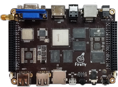
The development platform used to carry out our performance analysis will be the Firefly-RK3288 which is an all-in-one high performance multi-core computing platform based on the Rockchip RK3288 SoC featuring an ARM® Cortex®-A17 @1.8GHz and ARM® Mali™-T760 (Mali GPU Driver: r6p0-02rel0).
For all performance evaluations, DVFS has been disabled and the GPU clock has been set at the maximum frequency of 600MHz.
Further information about the development platform can be found at:
- Firefly | Focus on establish an open source platform based on cutting-edge technology
- Firefly-RK3288 – Mali Developer Center
Implementation
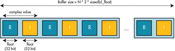
Let’s take a look at how we store our complex values. The input and output data are sorted into a floating point complex array with 2*N elements where the real and imaginary parts are placed alternately. Two different buffers with 2*N elements have been used to store the input and output values.
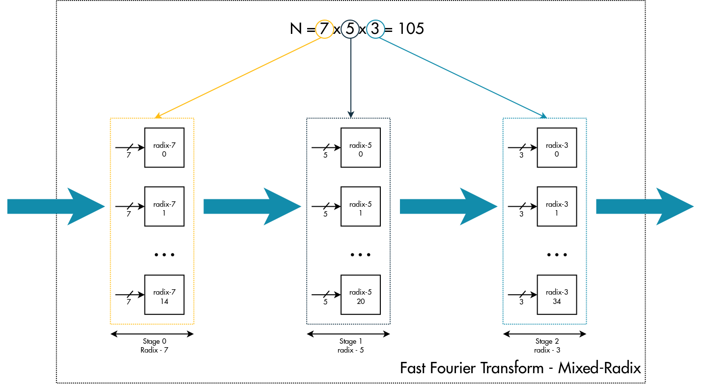
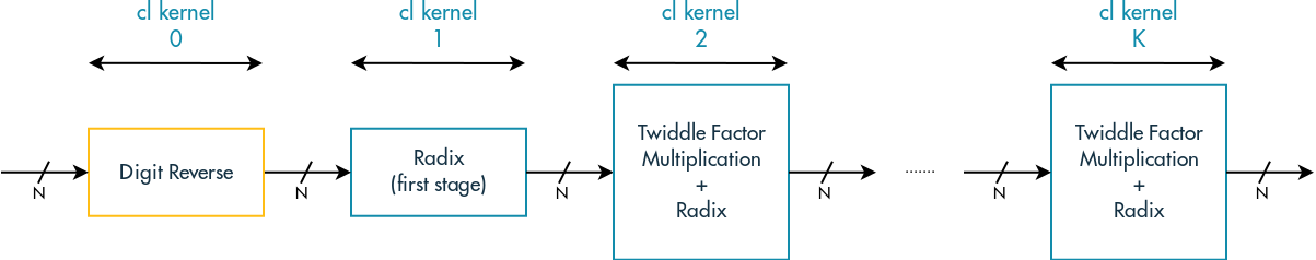
The FFT mixed-radix pipeline that we are going to study is composed mainly of 3 computation blocks:
- Digit-reverse
- Twiddle factor multiplication
- Radix computation

Indexing scheme
The only real complexity of FFT mixed-radix is the indexing scheme. The indexing scheme expresses the relation between the index n and k between 2 generic stages X and Y. This relation is fundamental because it allows for both knowing which input must be processed by each radix basic element and correctly performing the stages of digit reverse and twiddle factors multiplication.
Given 2 generic stages X and Y:
- n addresses the values in the stage X: n = nx + ny * Nx
- k addresses the values in the stage Y: k = ky + kx * Ny
with:
- nx = n % Nx, scans the columns – nx [0, Nx – 1]
- ny = floor(n / Nx), scans the rows – ny [0, N / Nx – 1]
- kx = floor(k / Ny), scans the rows – kx [0, N / Ny – 1]
- ky = (k % Ny), scans the columns – ky [0, Ny – 1]
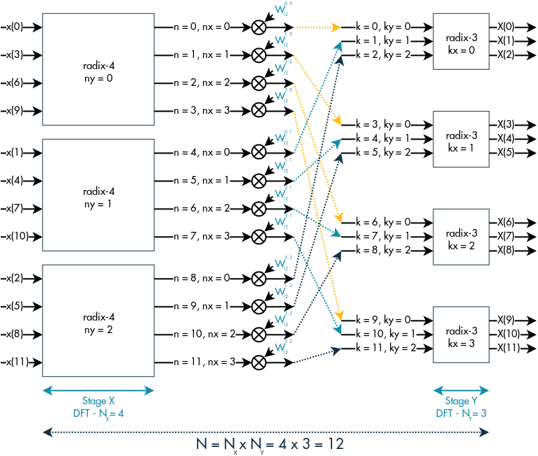
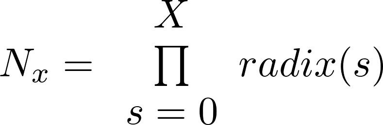
From the above picture we can easily see what nx, ny, kx and ky are. For what concerns Nx and Ny, in the case of just 2 radix stages they are respectively the radix order of stage X and Y. In the case of more than 2 radix stages, Ny is still the radix order of stage Y but Nx becomes the radix products from the first radix stage to the radix stage X.
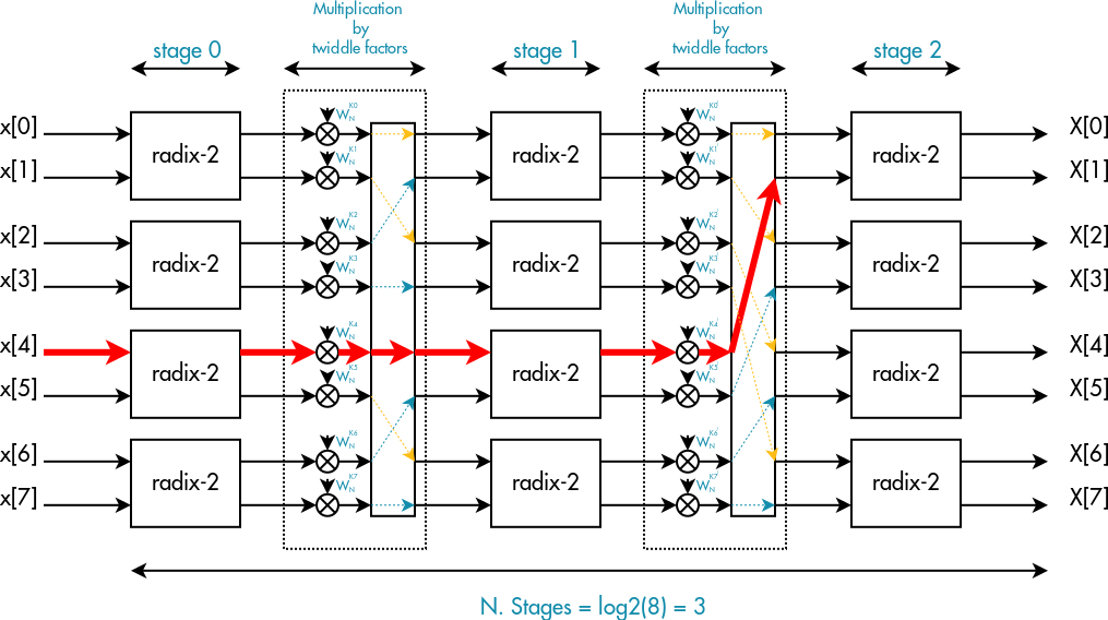
Nx is also known as span or butterfly span. The span is the offset between each complex input of radix basic element and it was introduced in the first article in reference to the radix-2 FFT algorithm.
i.e.
Let’s assume we have N = 8 x 4 x 4 x 3 x 2 (5 stages).
If the stages X and Y were stage 2 and stage 3, Nx would be Nx = 8 x 4 x 4 = 128 and Ny = 3
With a pipeline made up of M radix stages, we would like to have a relation between the index k and n between 2 generic stages, in particular we would like to have something like:
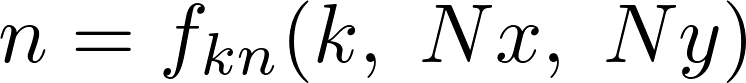
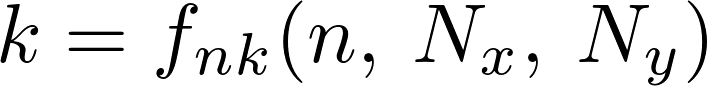
The general expressions for computing these mapping functions are:

where Ni is:

/**
* @brief Map index k to index n
*
* @param[in] k Index k
* @param[in] Nx It is the span
* @param[in] Ny It is the radix order of stage Y
*
* @return Index n
*/
uint map_k_to_n(uint k, uint Nx, uint Ny)
{
uint Ni = Nx * Ny;
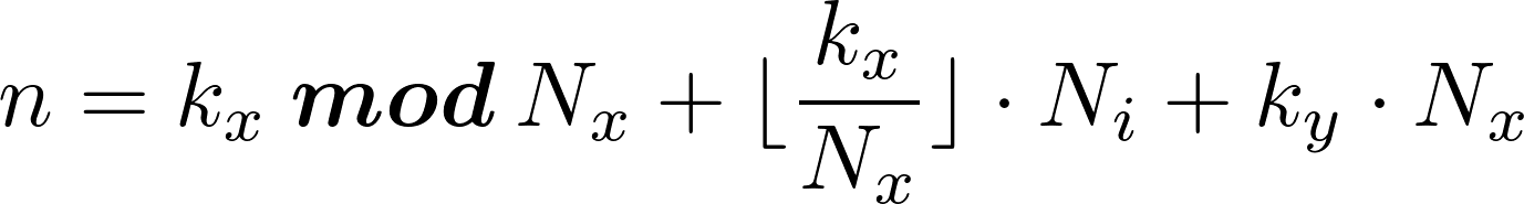
uint ky = k % Ny; // Remainder
uint kx = k / Ny; // Integer part
uint n = (kx % Nx) + (kx / Nx) * Ni + ky * Nx;
return n;
}
/**
* @brief Map index n to index k
*
* @param[in] n Index n
* @param[in] Nx It is the span
* @param[in] Ny It is the radix order of stage Y
*
* @return Index k
*/
uint map_n_to_k(uint n, uint Nx, uint Ny)
{
uint Ni = Nx * Ny;
uint k = (n * Ny) % Ni + (n / Nx) % Ny + Ni * (n / Ni);
return k;
}
Every time we compute a radix stage, it is good to keep the span Nx update.
/* Init Nx to 1 */
uint Nx = 1;
/* Scan each radix stage */
for(uint s = 0; s < n_stages; ++s)
{
/* Get radix order of stage s */
uint Ny = radix[s];
/* Body for computing twiddle factor multiplication and radix computation */
…
/* Update Nx */
Nx *= Ny;
}
Digit-reverse
Once we have introduced the indexing scheme, we are ready to analyze the main computation blocks of our pipeline. Let’s start with the digit-reverse.
The digit-reverse is the first stage of our pipeline, which places the input elements in a specific order called “digit-reverse order”.
The digit-reverse order would be exactly the order of the output elements if we left the input elements in linear order (0, 1, 2,…).
Since we know the relation between the index n and k, a possible way of knowing the digit-reverse order may be to iterate the mapping function map_n_to_k() from the first to the last stage in order to know how the input index n would be mapped at the end.
/**
* @brief This function computes the digit reverse index for each input
*
* @param[in] stage It contains the radix order for each radix stage
* @param[out] idx_digit_reverse It contains the digit-reverse order index
* @param[in] n_stages Total number of radix stages
* @param[in] N Number of input
*/
int digit_reverse(float* stage, uint* idx_digit_reverse, uint n_stages, uint N)
{
/* Scan elements */
for(uint n = 0; n < N; ++n)
{
uint k = n;
uint Nx = stage[0];
/* Scan stages */
for (uint s = 1; s < n_stages; ++s)
{
/* radix of stage s-th */
uint Ny = stage[s];
uint Ni = Ny * Nx;
/* Update k index */
k = (k * Ny) % Ni + (k / Nx) % Ny + Ni * (k / Ni);
/* Update Nx */
Nx *= Ny;
}
/* K is the index of digit-reverse */
idx_digit_reverse[n] = k;
}
}
Once we know the digit-reverse index, we can implement a CL kernel that places the input values in the required order.
/**
* @brief This kernel stores the input in digit-reverse order
*
* @param[in] input It contains the input complex values in linear order
* @param[out] output It contains the output complex values in digit-reverse order
* @param[in] idx_bit_reverse It contains the digit-reverse order index
*/
kernel void digit_reverse(global float2* input, global float2* output, global uint* idx_digit_reverse)
{
/* Each work-item stores a single complex values */
const uint n = get_global_id(0);
/* Get digit-reverse index */
const uint idx = idx_digit_reverse[n];
/* Get complex value */
float2 val = (float2)(input[idx]);
/* Store complex value */
output[n] = val;
}
The digit-reverse kernel uses 2 different cl_buffers:
- one for loading the input complex values
- one for storing the output complex values in digit-reverse order.
Twiddle Factor Multiplication
Twiddle factor multiplication is the intermediate stage between 2 generic radix stages X and Y. In particular it multiplies all the N output complex elements of radix stage X by a specific trigonometric complex constant before passing those values to the next stage Y.
This trigonometric complex constant -the “twiddle” factor – depends on nx and ky:
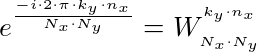
Even the twiddle factor multiplication is highly parallelizable and can be implemented by means of OpenCL in the following manner:
#define M_2PI_F 6.283185482025146484375f
#define TWIDDLE_FACTOR_MULTIPLICATION(phi, input) \
{ \
float2 w, tmp; \
w.x = cos(phi); \
w.y = sin(phi); \
tmp.x = (w.x * input.x) – (w.y * input.y); \
tmp.y = (w.x * input.y) + (w.y * input.x); \
input = tmp; \
}
/**
* @brief This kernel computes the twiddle factor multiplication between 2 generic radix stages X and Y
*
* @param[in, out] input It contains the input and output complex values
* @param[in] Nx It is the span
* @param[in] Ny It is the radix order of stage Y
* @param[in] Ni Nx * Ny
*/
kernel void twiddle_factor_multiplication(global float2* input, const uint Nx, const uint Ny, const uint Ni)
{
/* Each work-item computes a single complex input */
const uint n = get_global_id(0);
/* Compute nx */
uint nx = n % Nx;
/* Compute k index */
uint k = (n * Ny) % Ni + (n / Nx) % Ny + Ni * (n / Ni);
/* Compute ky */
uint ky = k % Ny;
/* Compute angle of twiddle factor */
float phi = (-M_2PI_F * nx * ky) / (float)Ni;
/* Multiply by twiddle factor */
TWIDDLE_FACTOR_MULTIPLICATION(phi, input[n]);
}
The above kernel uses the same cl_buffer for loading and storing.
An interesting optimization concerns the computation of ky. As we know,
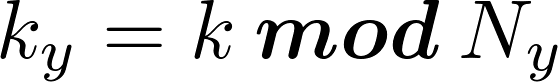
so:

since in the above expression A and B are multiples of Ny, the terms 1 and 3 will be 0 therefore:
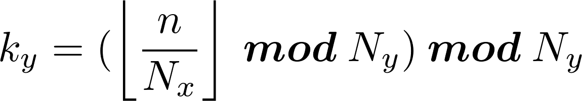
but for the identity property of the modulo operator we have:

and then we can compute ky as:
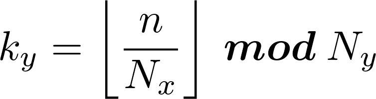
At this point we can simplify our OpenCL kernel in the following manner:
kernel void twiddle_factor_multiplication(global float2* input, const uint Nx, const uint Ny, const uint Ni)
{
/* Each work-item computes a single complex input */
const uint n = get_global_id(0);
/* Compute nx */
uint nx = n % Nx;
/* Compute ky */
uint ky = (n / Nx) % Ny; // <-
/* Compute angle of twiddle factor */
float phi = (-M_2PI_F * nx * ky) / (float)Ni;
/* Multiply by twiddle factor */
TWIDDLE_FACTOR_MULTIPLICATION(phi, input[n]);
}
Another important and simple optimization that we can introduce concerns the computation of the angle for the twiddle factor multiplication. As we can observe, the term (-M_2PI_F / (float)Ni) is a constant for all work-items and can therefore be passed as a argument to the CL kernel.
/**
* @brief This kernel computes the twiddle factor multiplication between 2 generic radix stages X and Y
*
* @param[in, out] input It contains the input and output complex values
* @param[in] Nx It is the span
* @param[in] Ny It is the radix order of stage Y
* @param[in] Ni Nx * Ny
* @param[in] exp_const (-M_2PI_F / (float)Ni)
*/
kernel void twiddle_factor_multiplication(global float2* input, const uint Nx, const uint Ny, const uint Ni, const float exp_const)
{
/* Each work-item computes a single complex input */
const uint n = get_global_id(0);
/* Compute nx */
uint nx = n % Nx;
/* Compute ky */
uint ky = (n / Nx) % Ny;
/* Compute angle of twiddle factor */
float phi = (float)(nx * ky) * exp_const; // <-
/* Multiply by twiddle factor */
TWIDDLE_FACTOR_MULTIPLICATION(phi, input[n]);
}
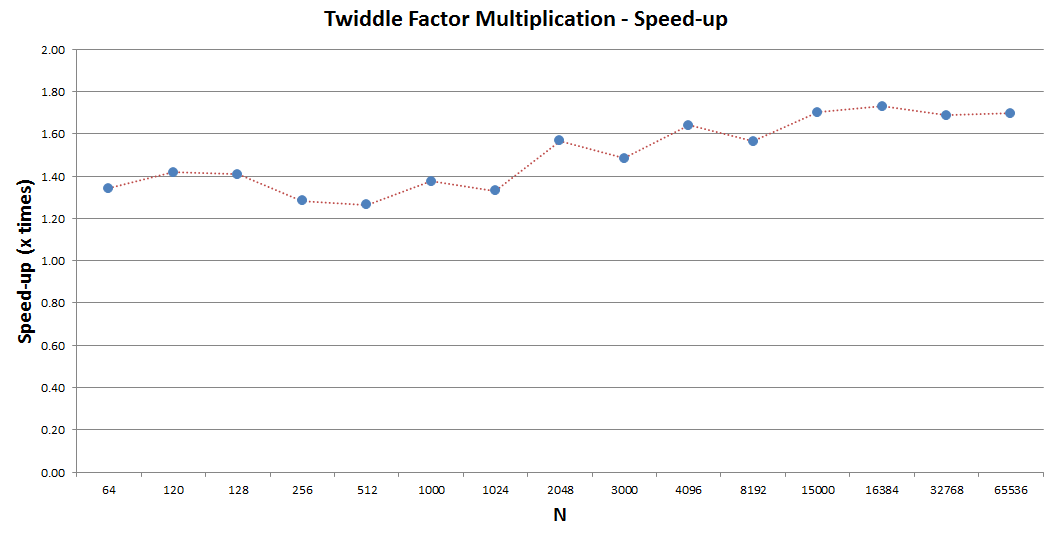
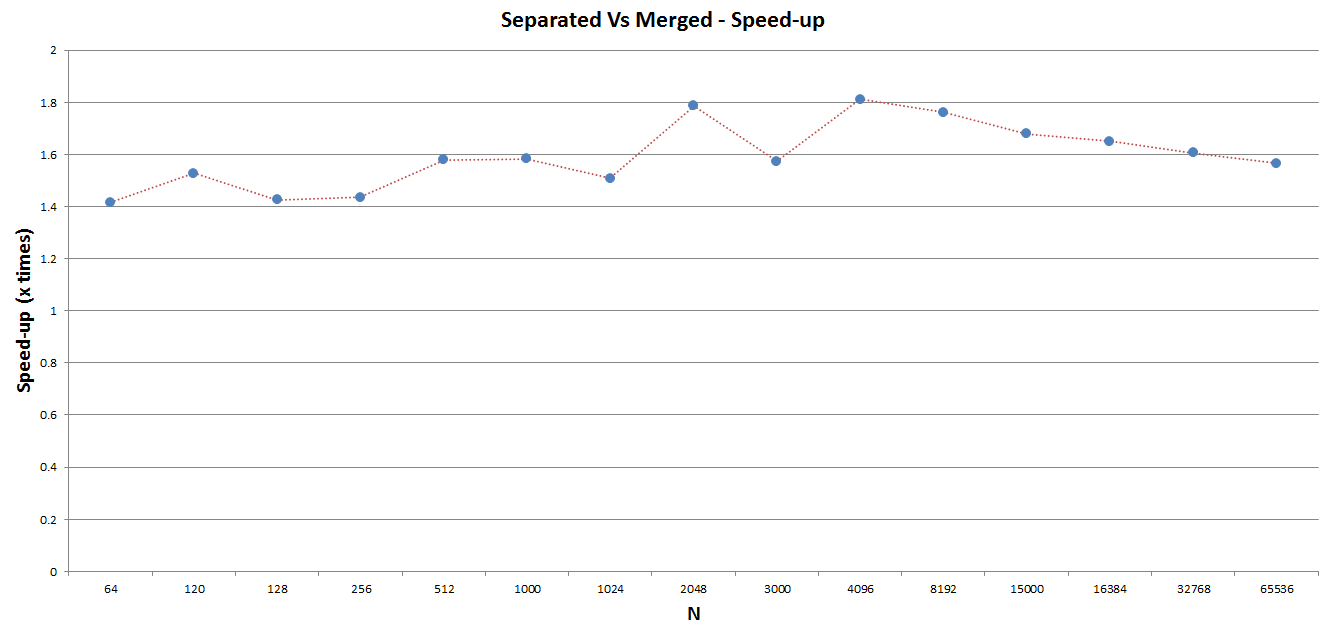
With these 2 simple optimizations, we are able to improve the performance of this kernel by a factor of ~1.6/1.7x as illustrated in the following graph.
Radix computation
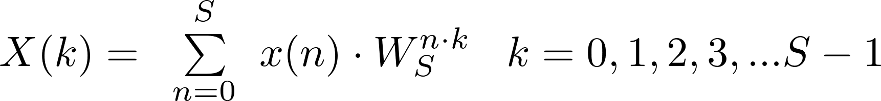
The radix stage is the main computation block of the pipeline composed of N / S radix-S basic elements.
Each radix-S consists of S inputs and S outputs and computes an optimized DFT of length S.
Since there is not a dependency between each radix basic element of the same stage, even the radix stage is an embarrassingly parallel problem.
In our implementation each radix-S of the same radix stage is performed by a single work-item. As in the first stage the radix basic element takes the input in linear order whilst for the following stages accordingly with the span Nx, we are going to use 2 different kernels for the radix basic element:
- One kernel for the first stage, which takes the input in linear order
- One kernel for the other radix stages
Both kernels use a single cl_buffer for loading and storing.
In the following we are going to describe the implementation of radix 2/3/4/5/7.
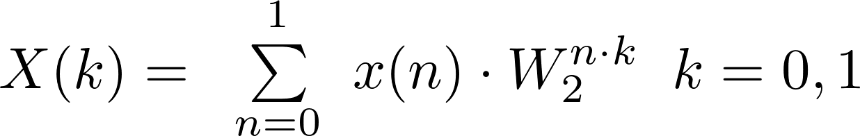
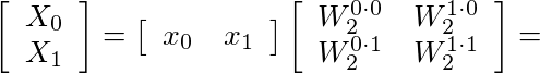
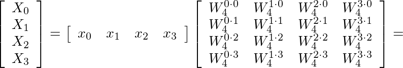
Radix-2
Defined as:
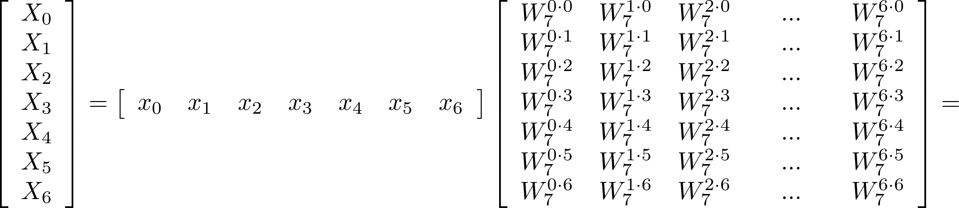
can be expressed in the following matrix form:
#define DFT_2(c0, c1) \
{ \
float2 v0; \
v0 = c0; \
c0 = v0 + c1; \
c1 = v0 – c1; \
}
/**
* @brief This kernel computes DFT of size 2 for the first stage
*
* @param[in, out] input It contains the input and output complex values
*/
kernel void radix_2_first_stage(global float* input)
{
/* Each work-item computes a single radix-2 */
uint idx = get_global_id(0) * 4;
/* Load two complex input values */
float4 in = vload4(0, input + idx);
/* Compute DFT N = 2 */
DFT_2(in.s01, in.s23);
/* Store two complex output values */
vstore4(in, 0, input + idx);
}
/**
* @brief This kernel computes DFT of size 2 for the radix stages after the first
*
* @param[in, out] input It contains the input and output complex value
* @param[in] Nx It is the span
* @param[in] Ni Nx * Ny
*/
kernel void radix_2(global float2* input, uint Nx, uint Ni)
{
/* Each work-item computes a single radix-2 */
uint kx = get_global_id(0);
/* Compute n index */
uint n = (kx % Nx) + (kx / Nx) * Ni;
/* Load two complex input values */
float2 c0 = input[n];
float2 c1 = input[n + Nx];
/* Compute DFT N = 2 */
DFT_2(c0, c1);
/* Store two complex output values */
input[n] = c0;
input[n + Nx] = c1;
}
Radix-3
Defined as:
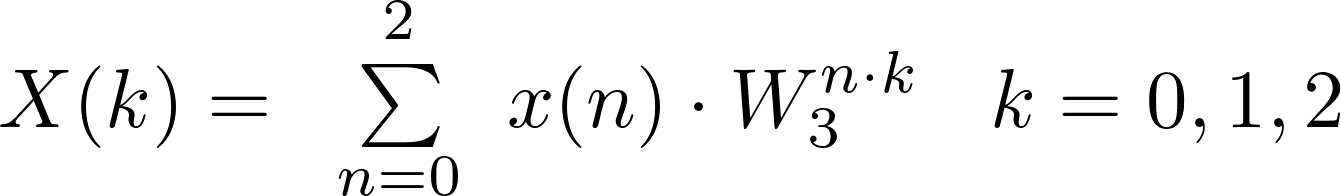
can be expressed in the following matrix form:
#define SQRT3DIV2 0.86602540378443f
#define DFT_3(c0, c1, c2) \
{ \
float2 v0 = c1 + c2; \
float2 v1 = c1 – c2; \
c1.x = c0.x – 0.5f * v0.x + v1.y * SQRT3DIV2; \
c1.y = c0.y – 0.5f * v0.y – v1.x * SQRT3DIV2; \
c2.x = c0.x – 0.5f * v0.x – v1.y * SQRT3DIV2; \
c2.y = c0.y – 0.5f * v0.y + v1.x * SQRT3DIV2; \
c0 = c0 + v0; \
}
/**
* @brief This kernel computes DFT of size 3 for the first stage
*
* @param[in, out] input It contains the input and output complex values
*/
kernel void radix_3_first_stage(global float* input)
{
/* Each work-item computes a single radix-3 */
uint idx = get_global_id(0) * 6;
/* Load three complex input values */
float4 in0 = vload4(0, input + idx);
float2 in1 = vload2(0, input + idx + 4);
/* Compute DFT N = 3 */
DFT_3(in0.s01, in0.s23, in1.s01);
/* Store three complex output values */
vstore4(in0, 0, input + idx);
vstore2(in1, 0, input + idx + 4);
}
/**
* @brief This kernel computes DFT of size 3 for the radix stages after the first
*
* @param[in, out] input It contains the input and output complex value
* @param[in] Nx It is the span
* @param[in] Ni Nx * Ny
*/
kernel void radix_3(global float2* input, uint Nx, uint Ni)
{
/* Each work-item computes a single radix-3 */
uint kx = get_global_id(0);
/* Compute n index */
uint n = (kx % Nx) + (kx / Nx) * Ni;
/* Load three complex input values */
float2 c0 = input[n];
float2 c1 = input[n + Nx];
float2 c2 = input[n + 2 * Nx];
/* Compute DFT N = 3 */
DFT_3(c0, c1, c2);
/* Store three complex output values */
input[n] = c0;
input[n + Nx] = c1;
input[n + 2 * Nx] = c2;
}
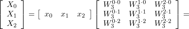
Radix-4
Defined as:
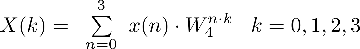
can be expressed in the following matrix form:
#define DFT_4(c0, c1, c2, c3) \
{ \
float2 v0, v1, v2, v3; \
v0 = c0 + c2; \
v1 = c1 + c3; \
v2 = c0 – c2; \
v3.x = c1.y – c3.y; \
v3.y = c3.x – c1.x; \
c0 = v0 + v1; \
c2 = v0 – v1; \
c1 = v2 + v3; \
c3 = v2 – v3; \
}
/**
* @brief This kernel computes DFT of size 4 for the first stage
*
* @param[in, out] input It contains the input and output complex values
*/
kernel void radix_4_first_stage(global float* input)
{
/* Each work-item computes a single radix-4 */
uint idx = get_global_id(0) * 8;
/* Load four complex input values */
float8 in = vload8(0, input + idx);
/* Compute DFT N = 4 */
DFT_4(in.s01, in.s23, in.s45, in.s67);
/* Store four complex output values */
vstore8(in, 0, input + idx);
}
/**
* @brief This kernel computes DFT of size 4 for the radix stages after the first
*
* @param[in, out] input It contains the input and output complex value
* @param[in] Nx It is the span
* @param[in] Ni Nx * Ny
*/
kernel void radix_4(global float2* input, uint Nx, uint Ni)
{
/* Each work-item computes a single radix-4 */
uint kx = get_global_id(0);
/* Compute n index */
uint n = (kx % Nx) + (kx / Nx) * Ni;
/* Load four complex input values */
float2 c0 = input[n];
float2 c1 = input[n + Nx];
float2 c2 = input[n + 2 * Nx];
float2 c3 = input[n + 3 * Nx];
/* Compute DFT N = 4 */
DFT_4(c0, c1, c2, c3);
/* Store four complex output values */
input[n] = c0;
input[n + Nx] = c1;
input[n + 2 * Nx] = c2;
input[n + 3 * Nx] = c3;
}
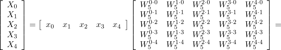
Radix-5
Defined as:
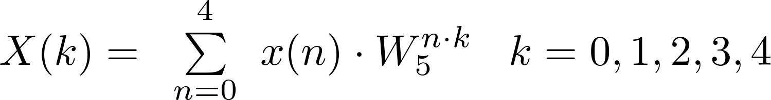
can be expressed in the following matrix form:
#define W5_A 0.30901699437494f
#define W5_B 0.95105651629515f
#define W5_C 0.80901699437494f
#define W5_D 0.58778525229247f
#define DFT_5(c0, c1, c2, c3, c4) \
{ \
float2 v0, v1, v2, v3, v4; \
v0 = c0; \
v1 = W5_A * (c1 + c4) – W5_C * (c2 + c3); \
v2 = W5_C * (c1 + c4) – W5_A * (c2 + c3); \
v3 = W5_D * (c1 – c4) – W5_B * (c2 – c3); \
v4 = W5_B * (c1 – c4) + W5_D * (c2 – c3); \
c0 = v0 + c1 + c2 + c3 + c4; \
c1 = v0 + v1 + (float2)(v4.y, -v4.x); \
c2 = v0 – v2 + (float2)(v3.y, -v3.x); \
c3 = v0 – v2 + (float2)(-v3.y, v3.x); \
c4 = v0 + v1 + (float2)(-v4.y, v4.x); \
}
/**
* @brief This kernel computes DFT of size 5 for the first stage
*
* @param[in, out] input It contains the input and output complex values
*/
kernel void radix_5_first_stage(global float* input)
{
/* Each work-item computes a single radix-5 */
uint idx = get_global_id(0) * 10;
/* Load five complex input values */
float8 in0 = vload8(0, input + idx);
float2 in1 = vload2(0, input + idx + 8);
/* Compute DFT N = 5 */
DFT_5(in0.s01, in0.s23, in0.s45, in0.s67, in1.s01);
/* Store five complex output values */
vstore8(in0, 0, input + idx);
vstore2(in1, 0, input + idx + 8);
}
/**
* @brief This kernel computes DFT of size 5 for the radix stages after the first
*
* @param[in, out] input It contains the input and output complex value
* @param[in] Nx It is the span
* @param[in] Ni Nx * Ny
*/
kernel void radix_5(global float2* input, uint Nx, uint Ni)
{
/* Each work-item computes a single radix-5 */
uint kx = get_global_id(0);
/* Compute n index */
uint n = (kx % Nx) + (kx / Nx) * Ni;
/* Load five complex input values */
float2 c0 = input[n];
float2 c1 = input[n + Nx];
float2 c2 = input[n + 2 * Nx];
float2 c3 = input[n + 3 * Nx];
float2 c4 = input[n + 4 * Nx];
/* Compute DFT N = 5 */
DFT_5(c0, c1, c2, c3, c4);
/* Store five complex output values */
input[n] = c0;
input[n + Nx] = c1;
input[n + 2 * Nx] = c2;
input[n + 3 * Nx] = c3;
input[n + 4 * Nx] = c4;
}
Radix-7
Defined as:
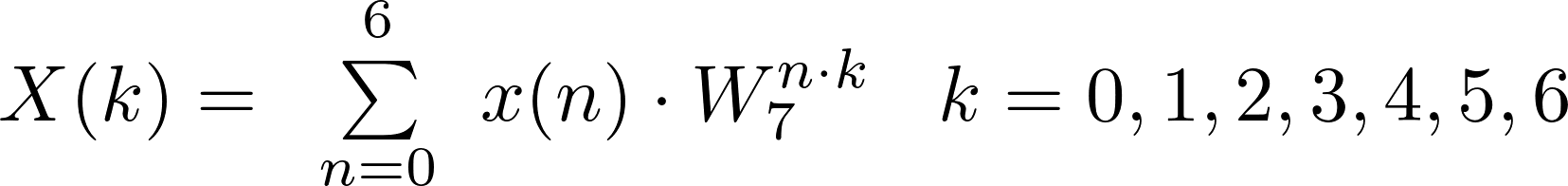
can be expressed in the following matrix form:
#define W7_A 0.62348980185873f
#define W7_B 0.78183148246802f
#define W7_C 0.22252093395631f
#define W7_D 0.97492791218182f
#define W7_E 0.90096886790241f
#define W7_F 0.43388373911755f
#define DFT_7(c0, c1, c2, c3, c4, c5, c6) \
{ \
float2 v0, v1, v2, v3, v4, v5, v6; \
v0 = c0; \
v1 = W7_A * (c1 + c6) – W7_C * (c2 + c5) – W7_E * (c3 + c4); \
v2 = W7_C * (c1 + c6) + W7_E * (c2 + c5) – W7_A * (c3 + c4); \
v3 = W7_E * (c1 + c6) – W7_A * (c2 + c5) + W7_C * (c3 + c4); \
v4 = W7_B * (c1 – c6) + W7_D * (c2 – c5) + W7_F * (c3 – c4); \
v5 = W7_D * (c1 – c6) – W7_F * (c2 – c5) – W7_B * (c3 – c4); \
v6 = W7_F * (c1 – c6) – W7_B * (c2 – c5) + W7_D * (c3 – c4); \
c0 = v0 + c1 + c2 + c3 + c4 + c5 + c6; \
c1 = v0 + v1 + (float2)(v4.y, -v4.x); \
c2 = v0 – v2 + (float2)(v5.y, -v5.x); \
c3 = v0 – v3 + (float2)(v6.y, -v6.x); \
c4 = v0 – v3 + (float2)(-v6.y, v6.x); \
c5 = v0 – v2 + (float2)(-v5.y, v5.x); \
c6 = v0 + v1 + (float2)(-v4.y, v4.x); \
}
/**
* @brief This kernel computes DFT of size 7 for the first stage
*
* @param[in, out] input It contains the input and output complex values
*/
kernel void radix_7_first_stage(global float* input)
{
/* Each work-item computes a single radix-7 */
uint idx = get_global_id(0) * 14;
/* Load seven complex input values */
float8 in0 = vload8(0, input + idx);
float4 in1 = vload4(0, input + idx + 8);
float2 in2 = vload2(0, input + idx + 12);
/* Compute DFT N = 7 */
DFT_7(in0.s01, in0.s23, in0.s45, in0.s67, in1.s01, in1.s23, in2.s01);
/* Store seven complex output values */
vstore8(in0, 0, input + idx);
vstore4(in1, 0, input + idx + 8);
vstore2(in2, 0, input + idx + 12);
}
/**
* @brief This kernel computes DFT of size 7 for the radix stages after the first
*
* @param[in, out] input It contains the input and output complex value
* @param[in] Nx It is the span
* @param[in] Ni Nx * Ny
*/
kernel void radix_7(global float2* input, uint Nx, uint Ni)
{
/* Each work-item computes a single radix-7 */
uint kx = get_global_id(0);
/* Compute n index */
uint n = (kx % Nx) + (kx / Nx) * Ni;
/* Load seven complex input values */
float2 c0 = input[n];
float2 c1 = input[n + Nx];
float2 c2 = input[n + 2 * Nx];
float2 c3 = input[n + 3 * Nx];
float2 c4 = input[n + 4 * Nx];
float2 c5 = input[n + 5 * Nx];
float2 c6 = input[n + 6 * Nx];
/* Compute DFT N = 7 */
DFT_7(c0, c1, c2, c3, c4, c5, c6);
/* Store seven complex output values */
input[n] = c0;
input[n + Nx] = c1;
input[n + 2 * Nx] = c2;
input[n + 3 * Nx] = c3;
input[n + 4 * Nx] = c4;
input[n + 5 * Nx] = c5;
input[n + 6 * Nx] = c6;
}
Merging twiddle factor multiplication with radix stage
Generally there are a couple of important benefits to combining 2 OpenCL kernels into one:
- fewer GPU jobs to dispatch thus reducing a possible driver overhead. In our implementation we are going to have (log2(N) – 1)fewer GPU jobs
- fewer memory accesses which is a great thing not only for performance but also for power consumption
Regarding this last aspect, we can easily guess that, since both twiddle factor multiplication and radix computation use the same cl_buffer for loading and storing, if we had 2 separated kernels we would access the same memory location twice.
Combining these 2 kernels, the new pipeline becomes:
In order to compute the twiddle factor multiplication inside the radix kernel, we need just a small tweak as we can see, for instance, in the following radix-5 OpenCL kernel:
/**
* @brief This kernel computes DFT of size 5 for the radix stages after the first
*
* @param[in, out] input It contains the input and output complex value
* @param[in] Nx It is the span
* @param[in] Ni Nx * Ny
* @param[in] exp_const (-M_2PI_F / (float)Ni)
*/
kernel void radix_5(global float2* input, uint Nx, uint Ni, float exp_const)
{
/* Each work-item computes a single radix-5 */
uint kx = get_global_id(0);
/* Compute nx */
uint nx = kx % Nx; // <-
/* Compute n index */
uint n = nx + (kx / Nx) * Ni; // <-
/* Load five complex input values */
float2 c0 = input[n];
float2 c1 = input[n + Nx];
float2 c2 = input[n + 2 * Nx];
float2 c3 = input[n + 3 * Nx];
float2 c4 = input[n + 4 * Nx];
/* Compute phi */
float phi = (float)nx * exp_const; // <- Please note: there is not ky
/* Multiply by twiddle factor */
TWIDDLE_FACTOR_MULTIPLICATION(phi, c1);
TWIDDLE_FACTOR_MULTIPLICATION(2 * phi, c2);
TWIDDLE_FACTOR_MULTIPLICATION(3 * phi, c3);
TWIDDLE_FACTOR_MULTIPLICATION(4 * phi, c4);
/* Compute DFT N = 5 */
DFT_5(c0, c1, c2, c3, c4);
/* Store five complex output values */
input[n] = c0;
input[n + Nx] = c1;
input[n + 2 * Nx] = c2;
input[n + 3 * Nx] = c3;
input[n + 4 * Nx] = c4;
}
From the following graph we can notice that the speed-up becomes considerable (~1.5x) already for small N.
Mixed-Radix vs Radix-2
We are approaching the end of this second part but before we finish, we’d like to present a final comparison between mixed-radix and radix-2.
In the first article we introduced mixed-radix as the solution to efficiently overcoming the problem of N not being a power of 2. However if we had N power of 2, what would be the benefit of using mixed-radix rather than radix-2?
As we know, radix-2 is just a special case of mixed-radix. Since in our implementation we have the radix-4 as well, 2 consecutive radix-2 stages can be merged in a single radix-4 stage thus reducing:
- The number of radix stages to compute
- The number of memory accesses
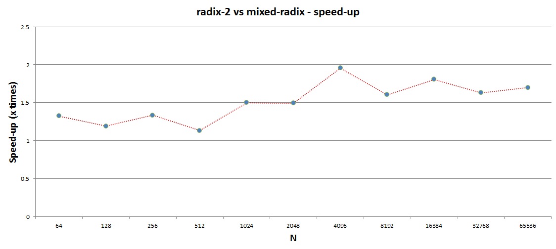
The following graph shows the speed-up achievable by mixed-radix with radix-4 against a pure radix-2 implementation. As we can appreciate, the speed-up is already considerable for small N getting 1.7x better performance for N greater than 4096.
Summary
In this second article we presented the implementation of the 3 main FFT mixed-radix computation blocks by means of OpenCL. Regarding the twiddle factor multiplications we showed how simple changes in CL kernels can significantly speed-up the computation.
We also saw that, although the nature of the pipeline is sequential, each stage represents an embarrassingly parallel problem that can be easily and efficiently implemented with OpenCL.
In the end, with the final comparison between mixed-radix and radix-2, we appreciated that mixed-radix not only provides the important flexibility in the choice of N but also provides a considerable speed-up with N power of 2 if we have the radix-4 as well.
In the next and final article of this blog series we are going to learn how to use the implemented FFT mixed-radix as a building block for computing the FFT for the case of 2 dimensions. This is mostly used in Image Processing, Computer Vision and Machine Learning applications.
Ciao,
Gian Marco Iodice
GPU Compute Software Engineer, ARM