
This blog post was originally published at Syntiant’s website. It is reprinted here with the permission of Syntiant.
Academic machine learning requires extensive toolsets for model training and evaluation, but the vast majority of academic work is more grounded in model capacity than looking at the energy cost of deploying those models. This puts modelers at a disadvantage for developing consumer device solutions. With a comparatively limitless power budget, modelers in the cloud have moved beyond thinking in terms of microwatts (uW). In the absence of an intuitive understanding for power tradeoffs, system designs are often negotiated between teams of machine learning and embedded engineers that don’t speak the same language. We want to help modelers arrive at the best solution possible without needing an electrical engineering degree.
The first step is understanding energy and power: energy is a measure of the capacity to perform a task (i.e., do “work”), while power is the rate at which energy is used over time. You can find the energy per inference as a metric for a network, and then apply the inference per second rate to find the average power consumed over time. A simple example would be a 60 watt (W) lightbulb. One second is 60 joules of energy for the lightbulb, averaging 60W of power. If you turn the light bulb off for half the day, the average power over a 24-hour period would only be 30W. The specific equation for watts is energy per second:
Power (watts) = Energy (joules) / Time (seconds)
More recent innovations have brought us LED lights, which can provide the same amount of light as a 60W incandescent bulb with only 6W of average power. All of a sudden you can supply the lights 10 times longer, or even put in 10 light bulbs for the same energy.
Battery powered devices provide another dimension, there is a limited amount of total energy that can be stored in a battery, and the total operating time is governed by the rate at which it is consumed. Battery capacity is typically reported at mW-hours (mWH), or sometimes in milliamp-hours (mAH) to specify how long the battery can continue to sustain an average power number. Going back to the light bulb, consider a light that could discharge 4 joules of energy over a 1 millisecond period, which is 4000W of peak power, but if you only do this 4 times a day, it is averaging 0.18W (or 180 mW) of power over the day.
More Efficient Light Bulbs
The ideal edge neural network (as exemplified by the Syntiant Neural Decision Processor™) combines the energy consumption of LED bulbs with the timing of a camera flashbulb: use less energy for the inference task and also run inferences only when needed. For any given task, the total energy consumed will be less.
The best way to quantify that is to look at the energy for an entire solution, and not just the peak performance reported by operations/watt (OPs/W). Many solutions that claim high OPs/W cannot sustain that performance over the duration of full networks. To fully evaluate a system, check the full system benchmarks like the TinyML Perf benchmark where Syntiant submitted the only solution with a neural processor. You can also pick well-known benchmark architectures like the Google-specified MobileNetV1 (alpha=0.25). Once you focus on the complete task, it removes the wiggle factor in partial information.
Example prompt for silicon providers: “Please fill out the following table for 0.25MobileNetV1 as specified by Google for RGB128x128 inputs.” These are the power performance results of the NDP200 running the quarter scale MobileNetV1, but what does this mean? How should we interpret this as modelers? Why do we want to know this? Let’s go row by row.
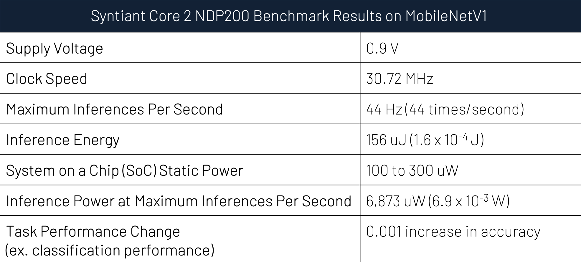
- Supply voltage and Clock Speed: In semiconductors, computations can be sped up by increasing the voltage, but the solution power is proportional to the square of the voltage. For example, moving from 0.9V to 1.1V comes with an almost 50% increase in power. This becomes an important tradeoff in solution design. You should provide just enough speed for the use-case, without increasing the supply voltage unnecessarily. Pushing the clock speed to 98 MHz increases throughput, but when increasing the volts to service the chip running faster you are making each individual inference more costly in terms of power. That voltage change makes a huge difference. You thus want your performance numbers to be presented at a consistent voltage and clock speed so you don’t buy a chip expecting the efficiencies of the low voltage and the throughput of the high voltage.
- Inference energy and Inference Power at Maximum Inferences Per Second: The combination of these two measures can tell you a lot about the numbers the silicon vendor is presenting. In an ideal case the inference power at maximum inferences per second should be (Maximum Inferences Per Second) * (Inference energy) because the chip should be able to duty cycle, which means it should only run when it is needed. However, when you are running so infrequently, the SoC static power begins to matter more than the Inference Power.
Tip: when you run one inference per second (i.e., 1 Hz), then the inference energy and power become interchangeable. You can think in terms of either 156 uJ or 156 uW.
- SoC Static Power: Semiconductors use more power when they are under load, but even when sitting idle there is a fixed cost associated with keeping the chip powered and clocking. The SoC static power answers the question, “presuming the chip already stores the neural network inputs and weights (i.e., they don’t need to be loaded from an external source), what are the power requirements not counting the cost of inference?” By stating the SoC static power explicitly, you will have the ability to know the power impacts of changes to the frame rates.
Framerate Math: With the inference energy and SoC Static Power estimates you are empowered to do back-of-the-envelope math for a variety of frame rates. The inference costs should scale approximately linearly, so running at 10 inferences per second will cost 1560 uW which is then added to the fixed cost of the SoC static power. These numbers are good enough to do solution design at the model level, but electrical engineering colleagues should be consulted to integrate other components of the solution power, such as the sensor power and memory transfer costs. Thankfully, these solution power elements typically don’t change in response to changing neural architectures. You can iterate model designs without constantly recalculating the sensor costs.
Solution Power = (SoC Static Power) + (Frame Rate)*(Inference Energy)
- Task Performance Change: Most silicon providers will not be running the neural architecture as provided by the public reference in its exact form. For example, the NDP200 allows you to select the numerical precision of activations. Depending on your selections, the task performance will change slightly. If you don’t ask for a task performance number, then the silicon will likely be running at its minimum resolution. Good luck solving the task at 1 bit weights, biases, and activations…
- Maximum Inferences Per Second: You need to know how often you can run the network since throughput in real-time applications is intimately related to task performance. (Our next post, “Duty Cycling for Modelers” will provide more insights on this.)
So now that you know the vital statistics of edge processors, how can these inform your neural architectures? In our next blog post, we will detail what may be affectionately called “Flash Bulb Solutions” as a way of spending neural capacity through time for massively efficient solutions.
Rouzbeh Shirvani, Ph.D., and Sean McGregor, Ph.D.
Machine Learning Architects, Syntiant