Quantization of Convolutional Neural Networks: Model Quantization

See “From Theory to Practice: Quantizing Convolutional Neural Networks for Practical Deployment” for the previous article in this series.

Significant progress in Convolutional Neural Networks (CNNs) has focused on enhancing model complexity while managing computational demands. Key advancements include efficient architectures like MobileNet¹, SqueezeNet², ShuffleNet³, and DenseNet⁴, which prioritize compute and memory efficiency. Further innovations involve quantizing weights and activations to lower precision, leading to approaches like Binary Neural Networks⁵, XNOR-net⁶, Ternary weight networks⁷ and many others^8-13.

The most common layers in CNNs are the convolution layer, batch-norm, activation, pooling and fully-connected layer. An example of a classifying CNN architecture is illustrated in Figure 1.

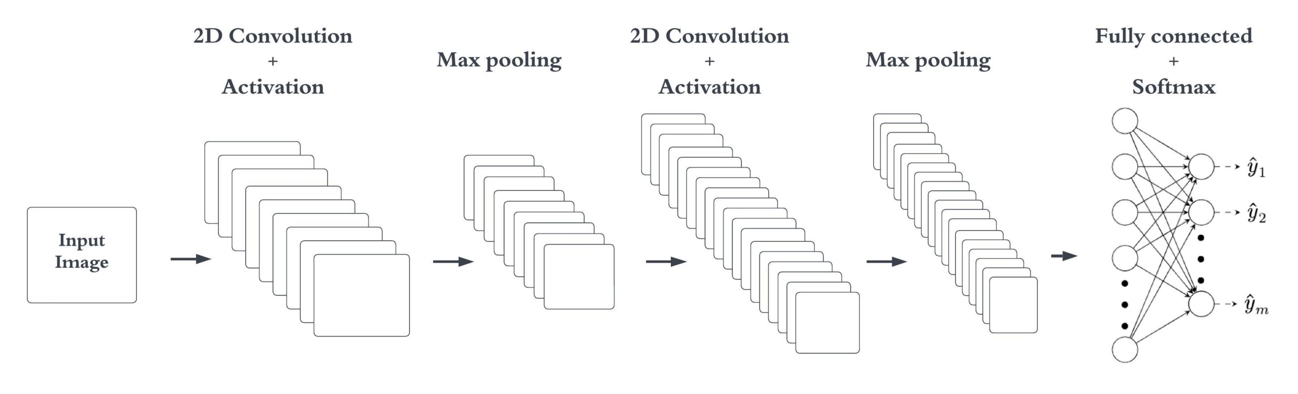
Figure 1. Overview of a 2D CNN

Quantization methods strike a balance between latency and accuracy, making them popular across diverse devices. Open-source tools like Pytorch, TFlite and ONNX now support 8-bit quantization for CNNs, addressing the critical need for portability and efficiency. While quantization schemes with fewer than 4 bits exhibit significant accuracy degradation and may not generalize well across different models, 8 and 4-bit quantization methods have become a popular choice. The preference for 8-bit quantization stems from native support on different edge devices. Table 1 summarizes the effects of quantization on model size and accuracy. The classification accuracy numbers are reported on the ImageNet dataset, and mostly show less than 1% drop in accuracy compared to the floating point version of the model¹⁴.

Network	FP32 Model Size	Top 1% Accuracy	Quant (INT8) Model Size	Top 1% Accuracy
AlexNet	233 MB	54.8	58 MB	54.68
VGG16	527.8MB	72.38	132.0 MB	72.32
InceptionV1	27 MB	67.23	10 MB	67.24
GoogleNet	27 MB	67.78	7 MB	67.73
ResNet50	97.8 MB	74.97	24.6 MB	74.77
DenseNet	32 MB	60.96	9 MB	60.2
SqueezeNet	5 MB	56.85	2 MB	56.48
MobileNet V2	13.3 MB	69.48	3.5 MB	68.3
ShuffleNet V2	8.79MB	66.35	2.28MB	66.15
EfficientNet	51.9 MB	80.4	13.0 MB	77.56

Table 1. Impact of 8-bit quantization on model size and accuracy¹⁴

Model Quantization

Model quantization techniques can be broadly classified into two main categories as shown in Figure 2.

Post-Training Quantization (PTQ)

This method quantizes a pre-trained model without retraining, offering a straightforward approach for quantizing the weights and the activations for deployment. Although PTQ can notably decrease model size, it may lead to some accuracy loss.

Quantization-Aware Training (QAT)

Quantization-Aware Training (QAT) integrates quantization considerations during the training process, potentially resulting in superior accuracy compared to PTQ. This approach is more complex and requires modifications to the training pipeline to accommodate quantization.

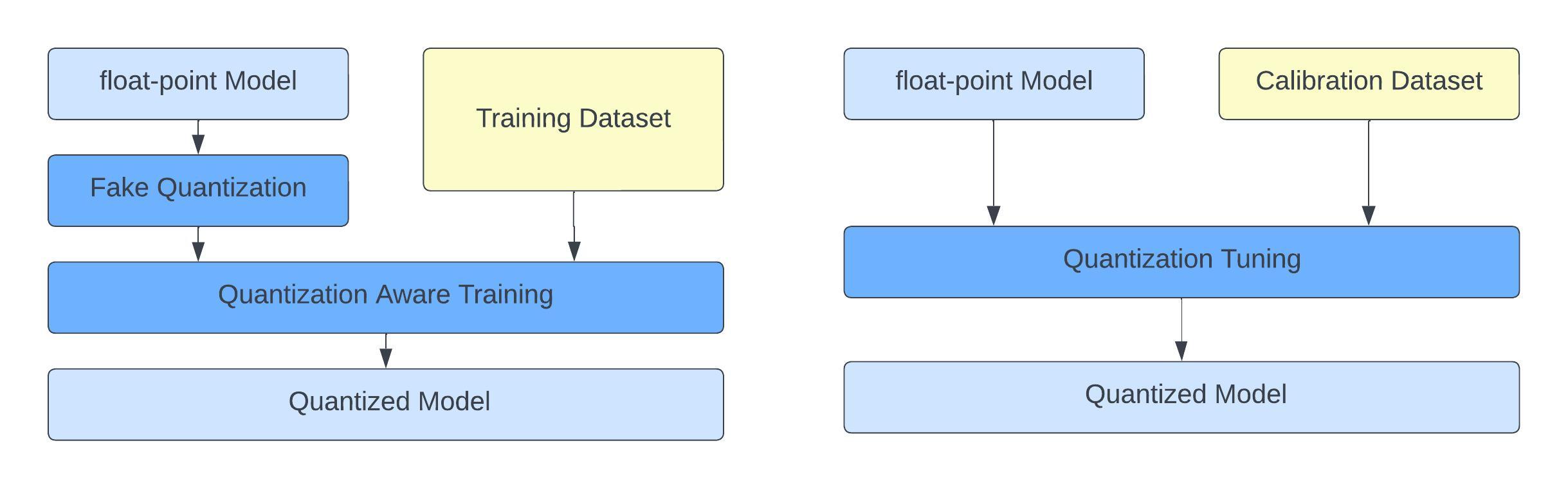
Figure 2. Comparison of Quantization Aware Training (QAT) on the left and Post Training Quantization (PTQ) on the right

Table 2 shows the results of image classification accuracy on the ImageNet dataset for PTQ and QAT.

Network	Float point	Symmetric , per-channel (Post Training Quantization)	Symmetric, per-channel (Quantization Aware Training)
Mobilenet-v1 1 224	0.709	0.591	0.707
Mobilenet-v2 1 224	0.719	0.698	0.711
Nasnet-Mobile	0.74	0.721	0.73
Mobilenet-v2 1.4 224	0.749	0.74	0.745
Inception-v3	0.78	0.78	0.78
Resnet-v1 50	0.752	0.751	0.75
Resnet-v2 50	0.756	0.75	0.75
Resnet-v1 152	0.768	0.762	0.762
Resnet-v2 152	0.778	0.76	0.76

Table 2. Accuracy results using QAT and PTQ on ImageNet dataset¹⁵

Quantization Scheme

Symmetric or asymmetric quantization schemes may be applied to either of or both the model’s weights and activations. Figure 3 shows a sample distribution of weights and activations of a trained network¹⁶.

Model Weights

After training, model weights often exhibit a symmetric and fixed distribution. In such cases, symmetric-per-channel quantization is commonly employed. This means that weights are quantized uniformly across different channels or dimensions.

Model Activations

In contrast, model activations vary based on the input images and features statistics, which can span a wider range and exhibit deviations. As a result, asymmetric-per-tensor quantization is often used for activations. This approach allows for more flexibility in handling the diverse  ranges of activation values.

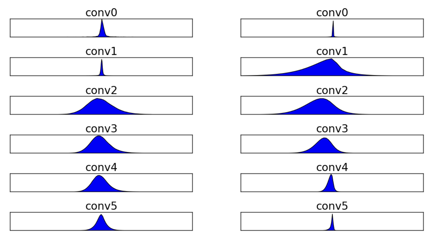
Figure 3. Histogram of distribution of weights and activations¹⁶

Quantization Granularity

At the heart of quantization granularity is the decision related to determining the quantization parameters for the different dimensions in the network, and the number of bits for representing the integer or the fixed-point values.

Per-layer/per-channel

Quantization strategies differ in their granularity: per-tensor assigns the same parameters to all values within a tensor, while per-channel allows different parameters for individual channels in a tensor. Per-channel quantization, tailored to the diversity of features within channels, often yields better accuracy. Choosing between these approaches depends on the model’s attributes and data. Per-channel quantization has shown promise in recovering lost accuracy in many commonly used models, making it popular in tools like PyTorch and TensorFlow. Table 3 shows the top 1% accuracy on ImageNet dataset using asymmetric quantization for activations with per-tensor and per-channel techniques.

Network	Float point	Asymmetric, per-layer	Asymmetric, per-channel
Mobilenet-v1 1 224	0.709	0.001	0.704
Mobilenet-v2 1 224	0.719	0.001	0.698
Nasnet-Mobile	0.74	0.722	0.74
Mobilenet-v2 1.4 224	0.749	0.004	0.74
Inception-v3	0.78	0.78	0.78
Resnet-v1 50	0.752	0.75	0.752
Resnet-v2 50	0.756	0.75	0.75
Resnet-v1 152	0.768	0.766	0.762
Resnet-v2 152	0.778	0.761	0.77

Table 3. Accuracy comparison between per-layer and per-channel quantization on ImageNet¹⁵

Bit-width

Opting for higher bit-widths like 16/32 ensures more accurate representation but increases memory and computational demands. Conversely, lower bit-widths like 4-bit or lower¹⁷ reduce resource usage but may sacrifice accuracy. The choice also considers tool chain and hardware support, making 8 bits representation a common choice for quantization.

Network	Bit-Width	Top 1% Accuracy	Top 5% Accuracy
AlexNet	32	56.5	79
	8	54.68	78.23
	3	54.2	77.6
	4	55.8	78.4
VGG-16	32	71.6	90.4
	8	72.32	90.97
	3	70.8	89.9
	4	71.4	90.3
ResNet18	32	69.8	89
	8	69.4	88.4
	3	68.9	88
	4	69.2	88.3
ResNet50	32	76.1	92.8
	8	74.77	92.32
	3	74.8	92.2
	4	75.9	92.7

Table 4. Comparison of  accuracy with different bit-widths¹⁷ on ImageNet dataset

Post Training Quantization

Post Training Quantization (PTQ) is the most popular approach for quantization as it is not resource intensive and only needs a small representative dataset to achieve acceptable results. PTQ is applied on pre-trained models, especially in cases where data is limited or hard to get. Recent studies have shown that PTQ without any calibration data is possible through synthetic data²⁰ or by using statistical knowledge of the network architecture¹⁸. Since it does not need any retraining, PTQ quantization is not resource intensive but may result in significant accuracy degradation.

Layer Fusion

Layer fusion, a common optimization for inference, combines convolution, batch normalization, and ReLU activations into one operation as shown in eq (1-3). Enabling this fusion before quantization reduces potential sources of quantization errors. This technique, also known as batchnorm constant folding, involves incorporating batch normalization parameters into convolutional layer weights and biases for efficiency. Activation functions like ReLU and ReLU6 are similarly fused to enhance inference efficiency by reducing data movement.

1. BatchNorm(w) = (w – μ2+ ϵ) + b
2. wfold = γw2 + ϵ
3. bfold = b – γ(2+ ϵ)

Calibration Dataset

The calibration dataset should reflect the expected data distribution during inference. The size of the calibration dataset should ensure diversity to represent inference input statistics accurately and prevent bias errors in the model. Research suggests that a calibration dataset of 100 to 1000 shuffled images is adequate to generalize classification accuracy^15,19 for a network trained on ImageNet which contains around 1 million images.

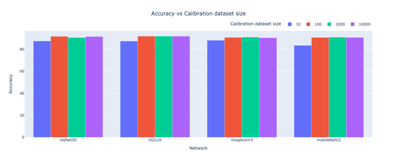
Figure 4. Effects of calibration dataset size on quantized model accuracy¹⁹

Quantization Aware Training

Quantization-Aware Training (QAT) addresses the risk of potential divergence from a converged state caused by quantization to a trained model. By emulating quantized inference during training through fake quantization nodes on weights and activations, QAT guides the model towards a convergence state optimized for quantization. Backpropagation still operates in float-point to avoid issues like diminishing gradients or high errors in low-precision scenarios²¹. Despite approximations, QAT significantly narrows the accuracy gap to less than 1% of floating-point results in various classification models.

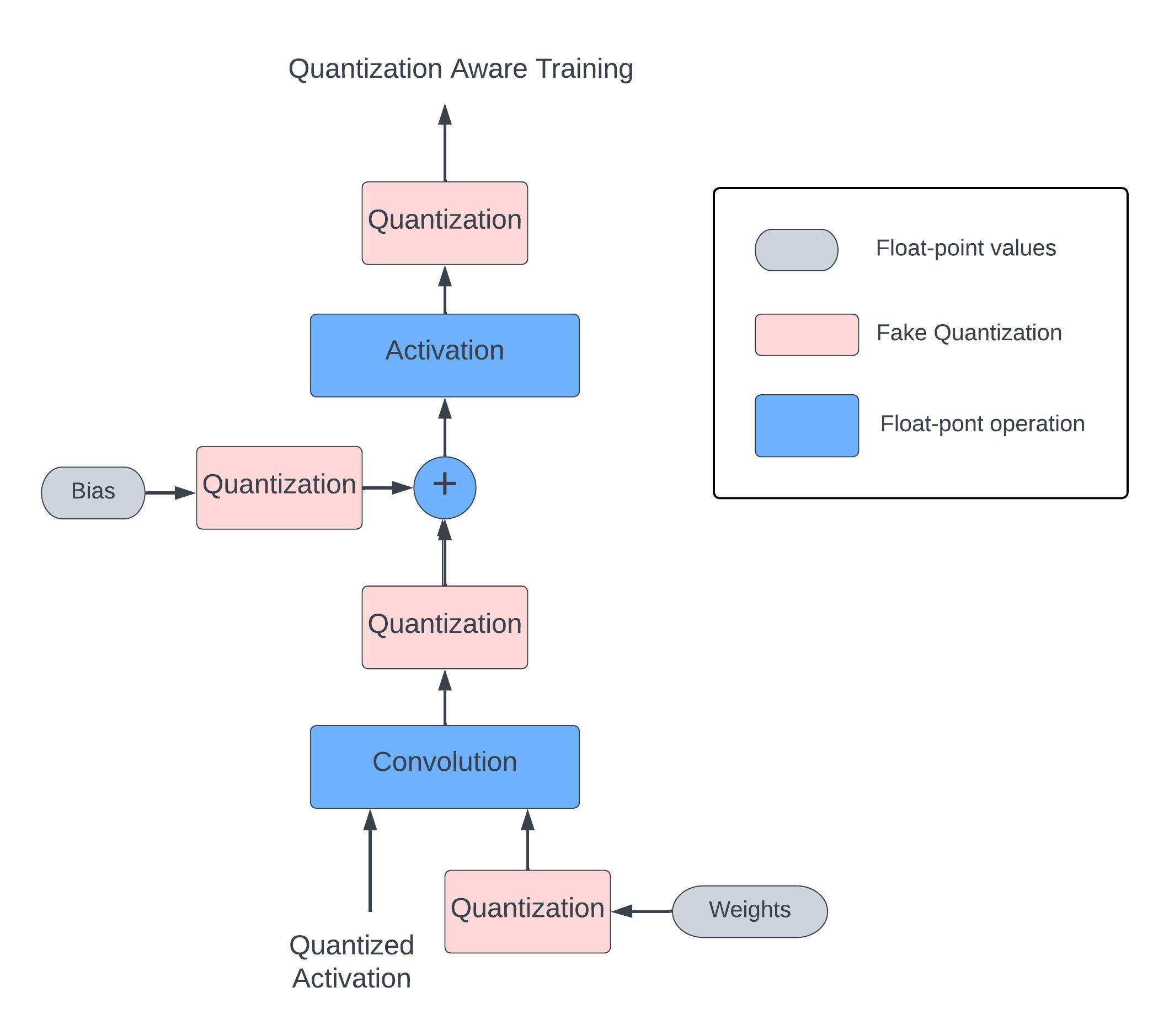
Figure 5. Shows simulation of quantization during QAT

More to Come

In a forthcoming article, we’ll explore the nuances of quantization error, examining various methods and tools for debugging and enhancing quantization accuracy. I’ll also discuss best practices for both quantization and optimizing performance.

Dwith Chenna
Senior Computer Vision Engineer, Magic Leap

References

1. A.G.Howard,M.Zhu,B.Chen,D.Kalenichenko,W.Wang, T. Weyand, M. Andreetto, and H. Adam. Mobilenets: Efficient convolutional neural networks for mobile vision appli- cations. CoRR, abs/1704.04861, 2017.
2. F. N. Iandola, M. W. Moskewicz, K. Ashraf, S. Han, W. J. Dally, and K. Keutzer. Squeezenet: Alexnet-level accuracy with 50x fewer parameters and¡ 1mb model size. arXiv preprint arXiv:1602.07360, 2016.
3. X. Zhang, X. Zhou, M. Lin, and J. Sun. Shufflenet: An extremely efficient convolutional neural network for mobile devices. CoRR, abs/1707.01083, 2017.
4. G. Huang, Z. Liu, L. van der Maaten, and K. Q. Wein- berger. Densely connected convolutional networks. In The IEEE Conference on Computer Vision and Pattern Recogni- tion (CVPR), July 2017.
5. I. Hubara, M. Courbariaux, D. Soudry, R. El-Yaniv, and Y. Bengio. Binarized neural networks. In Advances in neural information processing systems, pages 4107–4115, 2016.
6. M.Rastegari,V.Ordonez,J.Redmon,andA.Farhadi.Xnor- net: Imagenet classification using binary convolutional neural networks. arXiv preprint arXiv:1603.05279, 2016.
7. F. Li, B. Zhang, and B. Liu. Ternary weight networks. arXiv preprint arXiv:1605.04711, 2016.
8. S. Han, H. Mao, and W. J. Dally. Deep compression: Com- pressing deep neural network with pruning, trained quantiza- tion and huffman coding. CoRR, abs/1510.00149, 2, 2015.
9. C. Leng, H. Li, S. Zhu, and R. Jin. Extremely low bit neural network: Squeeze the last bit out with admm. arXiv preprint arXiv:1707.09870, 2017.
10. N. Mellempudi, A. Kundu, D. Mudigere, D. Das, B. Kaul, and P. Dubey. Ternary neural networks with fine-grained quantization. arXiv preprint arXiv:1705.01462, 2017.
11. A. Zhou, A. Yao, Y. Guo, L. Xu, and Y. Chen. Incremen- tal network quantization: Towards lossless cnns with low- precision weights. arXiv preprint arXiv:1702.03044, 2017.
12. S. Zhou, Y. Wu, Z. Ni, X. Zhou, H. Wen, and Y. Zou. Dorefa-net: Training low bitwidth convolutional neural networks with low bitwidth gradients. arXiv preprint arXiv:1606.06160, 2016.
13. C. Zhu, S. Han, H. Mao, and W. J. Dally. Trained ternary quantization. arXiv preprint arXiv:1612.01064, 2016.
14. Dwith Chenna, Evolution of Convolutional Neural Network(CNN): Compute vs Memory bandwidth for Edge AI, IEEE FeedForward Magazine 2(3), 2023, pp. 3-13.
15. Raghuraman Krishnamoorthi. Quantizing deep convolutional networks for efficient inference: A whitepaper. arXiv preprint arXiv:1806.08342, 2018.
16. D. Lin, S. Talathi, and S. Annapureddy. Fixed point quantization of deep convolutional networks. In the International Conference on Machine Learning, pages 2849–2858, 2016.
17. Banner, R., Nahshan, Y., Hoffer, E., and Soudry, D. (2019). Post-training 4-bit quantization of convolution networks for rapid-deployment.
18. Nagel, M., van Baalen, M., Blankevoort, T., and Welling, M. (2019). Data-free quantization through weight equalization and bias correction.
19. Dwith Chenna, “Quantization of Convolutional Neural Networks: A Practical Approach”, International Journal of Science & Engineering Development Research, Vol.8, Issue 12, page no.181 – 192, December-2023, Available :http://www.ijrti.org/papers/IJRTI2312025.pdf
20. Cai, Y., Yao, Z., Dong, Z., Gholami, A., Mahoney, M. W., and Keutzer, K. (2020). Zeroq: A novel zero shot quantization framework.
21. Matthieu Courbariaux, Yoshua Bengio, and JeanPierre David. BinaryConnect: Training deep neural networks with binary weights during propagations. In Advances in neural information processing systems, pages 3123–3131, 2015.