
This article was originally published at NVIDIA’s website. It is reprinted here with the permission of NVIDIA.
Starting with TensorRT 7.0, the Universal Framework Format (UFF) is being deprecated. In this post, you learn how to deploy TensorFlow trained deep learning models using the new TensorFlow-ONNX-TensorRT workflow. Figure 1 shows the high-level workflow of TensorRT.
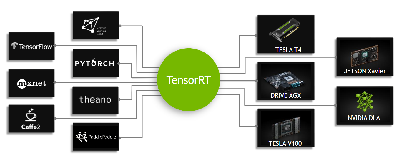
Figure 1. TensorRT is an inference accelerator.
First, a network is trained using any framework. After a network is trained, the batch size and precision are fixed (with precision as FP32, FP16, or INT8). The trained model is passed to the TensorRT optimizer, which outputs an optimized runtime also called a plan. The .plan file is a serialized file format of the TensorRT engine. The plan file needs to be deserialized to run inference using the TensorRT runtime.
To optimize models implemented in TensorFlow, the only thing you have to do is convert models to the ONNX format and use the ONNX parser in TensorRT to parse the model and build the TensorRT engine. Figure 2 shows the high-level ONNX workflow.
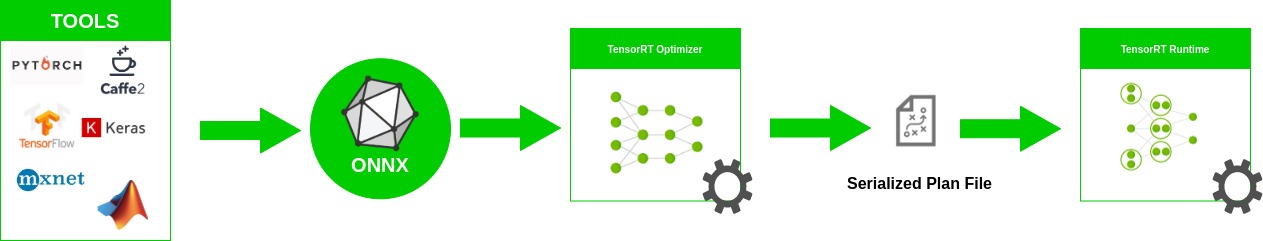
Figure 2. ONNX workflow.
In this post, we discuss how to create a TensorRT engine using the ONNX workflow and how to run inference from a TensorRT engine. More specifically, we demonstrate end-to-end inference from a model in Keras or TensorFlow to ONNX, and to a TensorRT engine with ResNet-50, semantic segmentation, and U-Net networks. Finally, we explain how you can use this workflow on other networks.
ONNX overview
ONNX is an open format for machine learning and deep learning models. It allows you to convert deep learning and machine learning models from different frameworks such as TensorFlow, PyTorch, MATLAB, Caffe, and Keras to a single format.
It defines a common set of operators, common sets of building blocks of deep learning, and a common file format. It provides a definition of a computation graph, as well as built-in operators. The list of ONNX nodes that may have one or more inputs or outputs forms an acyclic graph.
ResNet ONNX workflow example
In this example, we show how to use the ONNX workflow on two different networks and create a TensorRT engine. The first network is ResNet-50.
The workflow consists of the following steps:
- Convert the TensorFlow/Keras model to a .pb file.
- Convert the .pb file to the ONNX format.
- Create a TensorRT engine.
- Run inference from the TensorRT engine.
Converting the model to .pb
The first step is to convert the model to a .pb file. The following code example converts the ResNet-50 model to a .pb file:
import keras
from tensorflow.keras.models import Model
import keras.backend as K
K.set_learning_phase(0)

# load ResNet50 model pre-trained on imagenet
model = keras.applications.resnet.ResNet50(include_top=True, weights='imagenet', input_tensor=None, input_shape=None, pooling=None, classes=1000)

# Convert keras ResNet50 model to .bp file
in_tensor_name, out_tensor_names = keras_to_pb(model, "models/resnet50.pb", None)
In addition to Keras, you can also download ResNet-50 from the following locations:
- Deep Learning Examples GitHub repository: Provides the latest deep learning example networks. You can also see the ResNet-50 branch, which contains a script and recipe to train the ResNet-50 v1.5 model.
- NVIDIA NGC Models: It has the list of checkpoints for pretrained models. As an example, search on ResNet-50v1.5 for TensorFlow and get the latest checkpoint from the Download page.
def keras_to_pb(model, output_filename, output_node_names):

    """
    This is the function to convert the keras model to pb.

    Args:
       model: The keras model.
       output_filename: The output .pb file name.
       output_node_names: The output nodes of the network (if None,
       the function gets the last layer name as the output node).
    """

    # Get names of input and output nodes.
 in_name = model.layers[0].get_output_at(0).name.split(':')[0]

    if output_node_names is None:
        output_node_names = [model.layers[-1].get_output_at(0).name.split(':')[0]]

    sess = keras.backend.get_session()

    # TensorFlow freeze_graph expects a comma-separated string of output node names.
 output_node_names_tf = ','.join(output_node_names)

    frozen_graph_def = tf.graph_util.convert_variables_to_constants(
        sess,
        sess.graph_def,
        output_node_names)

    sess.close()
    wkdir = ''
 tf.train.write_graph(frozen_graph_def, wkdir, output_filename, as_text=False)

    return in_name, output_node_names
Converting the .pb file to ONNX
The second step is to convert the .pb model to the ONNX format. To do this, first install tf2onnx.
After installing tf2onnx, there are two ways of converting the model from a .pb file to the ONNX format. The first way is to use the command line and the second method is by using Python API. Run the following command:
python -m tf2onnx.convert --input /Path/to/resnet50.pb --inputs input_1:0 --outputs probs/Softmax:0 --output resnet50.onnx
Creating the TensorRT engine from ONNX
To create the TensorRT engine from the ONNX file, run the following command:
import tensorrt as trt

TRT_LOGGER = trt.Logger(trt.Logger.WARNING)
trt_runtime = trt.Runtime(TRT_LOGGER)
def build_engine(onnx_path, shape = [1,224,224,3]):

   """
   This is the function to create the TensorRT engine
   Args:
      onnx_path : Path to onnx_file.
      shape : Shape of the input of the ONNX file.
  """
   with trt.Builder(TRT_LOGGER) as builder, builder.create_network(1) as network, trt.OnnxParser(network, TRT_LOGGER) as parser:
       builder.max_workspace_size = (256 << 20)
       with open(onnx_path, 'rb') as model:
           parser.parse(model.read())
       network.get_input(0).shape = shape
       engine = builder.build_cuda_engine(network)
       return engine

def save_engine(engine, file_name):
   buf = engine.serialize()
   with open(file_name, 'wb') as f:
       f.write(buf)
def load_engine(trt_runtime, engine_path):
   with open(engine_path, 'rb') as f:
       engine_data = f.read()
   engine = trt_runtime.deserialize_cuda_engine(engine_data)
   return engine
This code example contains the following variable:
- max_workspace_size: Maximum GPU temporary memory that
ICudaEnginecan use at execution time.
The builder creates an empty network (builder.create_network()) and the ONNX parser parses the ONNX file into the network (parser.parse(model.read())). You set the input shape for the network (network.get_input(0).shape = shape), after which the builder creates the engine (engine = builder.build_cuda_engine(network)). To create the engine, run the following code example:
import engine as eng
import argparse
from onnx import ModelProto

 engine_name = “resnet50.plan”
 onnx_path = "/path/to/onnx/result/file/"
 batch_size = 1

 TRT_LOGGER = trt.Logger(trt.Logger.WARNING)
 trt_runtime = trt.Runtime(TRT_LOGGER)

 model = ModelProto()
 with open(onnx_path, "rb") as f:
    model.ParseFromString(f.read())

 d0 = model.graph.input[0].type.tensor_type.shape.dim[1].dim_value
 d1 = model.graph.input[0].type.tensor_type.shape.dim[2].dim_value
 d2 = model.graph.input[0].type.tensor_type.shape.dim[3].dim_value
 shape = [batch_size , d0, d1 ,d2]
 engine = eng.build_engine(onnx_path, shape= shape)
 eng.save_engine(engine, engine_name)
In this code example, you first get the input shape from the ONNX model. Next, create the engine, and then save the engine in a .plan file.
Running inference from the TensorRT engine:
The TensorRT engine runs inference in the following workflow:
- Allocate buffers for inputs and outputs in the GPU.
- Copy data from the host to the allocated input buffers in the GPU.
- Run inference in the GPU.
- Copy results from the GPU to the host.
- Reshape the results as necessary.
These steps are explained in detail in the following code examples:
 import tensorrt as trtimport pycuda.driver as cuda

def allocate_buffers(engine, batch_size, data_type):

   """
   This is the function to allocate buffers for input and output in the device
   Args:
      engine : The path to the TensorRT engine.
      batch_size : The batch size for execution time.
      data_type: The type of the data for input and output, for example trt.float32.

   Output:
      h_input_1: Input in the host.
      d_input_1: Input in the device.
      h_output_1: Output in the host.
      d_output_1: Output in the device.
      stream: CUDA stream.

   """

   # Determine dimensions and create page-locked memory buffers (which won't be swapped to disk) to hold host inputs/outputs.
   h_input_1 = cuda.pagelocked_empty(batch_size * trt.volume(engine.get_binding_shape(0)), dtype=trt.nptype(data_type))
   h_output = cuda.pagelocked_empty(batch_size * trt.volume(engine.get_binding_shape(1)), dtype=trt.nptype(data_type))
   # Allocate device memory for inputs and outputs.
   d_input_1 = cuda.mem_alloc(h_input_1.nbytes)

   d_output = cuda.mem_alloc(h_output.nbytes)
   # Create a stream in which to copy inputs/outputs and run inference.
   stream = cuda.Stream()
   return h_input_1, d_input_1, h_output, d_output, stream
The first two lines are for determining the dimensions for input and output. You create page-locked memory buffers in host (h_input_1, h_output). Then, you allocate device memory for input and output the same size as host input and output (d_input_1, d_output). The next step is to create the CUDA stream for copying data between the allocated memory from device and host.
import tensorrt as trt
import numpy as np
import pycuda.driver as cuda

def load_images_to_buffer(pics, pagelocked_buffer):

   preprocessed = np.asarray(pics).ravel()
   np.copyto(pagelocked_buffer, preprocessed)


def do_inference(engine, pics_1, h_input_1, d_input_1, h_output, d_output, stream, batch_size, height, width):

   """
   This is the function to run the inference
   Args:
      engine : Path to the TensorRT engine.
      pics_1 : Input images to the model.
      h_input_1: Input in the host.
      d_input_1: Input in the device.
      h_output_1: Output in the host.
      d_output_1: Output in the device.
      stream: CUDA stream.
      batch_size : Batch size for execution time.
      height: Height of the output image.
      width: Width of the output image.

   Output:
      The list of output images.

   """

   load_images_to_buffer(pics_1, h_input_1)

   with engine.create_execution_context() as context:
       # Transfer input data to the GPU.
       cuda.memcpy_htod_async(d_input_1, h_input_1, stream)

       # Run inference.

       context.profiler = trt.Profiler()
       context.execute(batch_size=1, bindings=[int(d_input_1), int(d_output)])

       # Transfer predictions back from the GPU.
       cuda.memcpy_dtoh_async(h_output, d_output, stream)
       # Synchronize the stream.
       stream.synchronize()
       # Return the host output.
       out = h_output.reshape((batch_size,-1, height, width))
       return out
In this code example, in the do_inference function, the first step is to load images to buffers in the host using the load_images_to_buffer function. Then the input data is transferred to the GPU (cuda.memcpy_htod_async(d_input_1, h_input_1, stream)) and inference is run using context.execute. Finally the results are copied from GPU to the host (cuda.memcpy_dtoh_async(h_output, d_output, stream)).
Semantic segmentation ONNX workflow example
In the post Fast INT8 Inference for Autonomous Vehicles with TensorRT 3, the author covered the process of UFF workflow for a semantic segmentation model.
In this post, you use similar networks to run the ONNX workflow for semantic segmentation. The network consists of a VGG16-based encoder and three upsampling layers implemented using a deconvolutional layer. The network is trained in about 40,000 iterations on the Cityscapes Dataset.
There are multiple ways of converting the TensorFlow model to an ONNX file. One way is the one explained in the ResNet50 section. Keras also has its own Keras-to-ONNX file converter. Sometimes, some of the layers are not supported in the TensorFlow-to-ONNX but they are supported in the Keras to ONNX converter. Depending on the Keras framework and the type of layers used, you may need to choose between converters.
In the following code example, you directly convert the Keras model to ONNX using the Keras-to-ONNX converter. Download the pretrained semantic segmentation file, semantic_segmentation.hdf5.
import keras
import tensorflow as tf
from keras2onnx import convert_keras

def keras_to_onnx(model, output_filename):
   onnx = convert_keras(model, output_filename)
   with open(output_filename, "wb") as f:
       f.write(onnx.SerializeToString())

semantic_model = keras.models.load_model('/path/to/semantic_segmentation.hdf5')
keras_to_onnx(semantic_model, 'semantic_segmentation.onnx')
Figure 3 shows the architecture of the network.
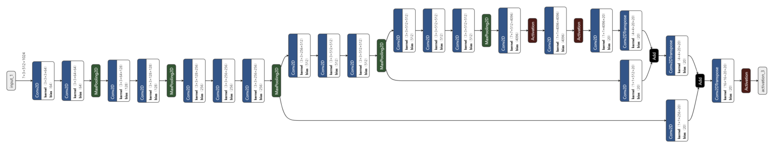
Figure 3. The VGG16-based semantic segmentation model.
As in the previous example, use the following code example to create the engine for semantic segmentation.
import engine as engfrom onnx import ModelProto
import tensorrt as trt


engine_name = 'semantic.plan'
onnx_path = "semantic.onnx"
batch_size = 1

TRT_LOGGER = trt.Logger(trt.Logger.WARNING)
trt_runtime = trt.Runtime(TRT_LOGGER)

model = ModelProto()
with open(onnx_path, "rb") as f:
  model.ParseFromString(f.read())

d0 = model.graph.input[0].type.tensor_type.shape.dim[1].dim_value
d1 = model.graph.input[0].type.tensor_type.shape.dim[2].dim_value
d2 = model.graph.input[0].type.tensor_type.shape.dim[3].dim_value
shape = [batch_size , d0, d1 ,d2]
engine = eng.build_engine(onnx_path, shape= shape)
eng.save_engine(engine, engine_name)
To test the output of the model, use the Cityscapes Dataset. To work with Cityscapes, you must have the following functions: sub_mean_chw and color_map. These functions also are used in the post, Fast INT8 Inference for Autonomous Vehicles with TensorRT 3.
In the following code example, sub_mean_chw is for subtracting the mean value from the image as the preprocessing step and color_map is the mapping from the class ID to a color. The latter is used for visualization.
import glob
from random import shuffle
import numpy as np
from PIL import Image
import tensorrt as trt
import labels  # from cityscapes evaluation script

MEAN = (71.60167789, 82.09696889, 72.30508881)
CLASSES = 19
CHANNEL = 3
HEIGHT = 512
WIDTH = 1024

def sub_mean_chw(data):
   data = data.transpose((1, 2, 0))  # CHW -> HWC
   data -= np.array(MEAN)  # Broadcast subtract
   data = data.transpose((2, 0, 1))  # HWC -> CHW
   return data

def rescale_image(image, output_shape, order=1):
   image = skimage.transform.resize(image, output_shape,
               order=order, preserve_range=True, mode='reflect')
   return image

def color_map(output):
   output = output.reshape(CLASSES, HEIGHT, WIDTH)
   out_col = np.zeros(shape=(HEIGHT, WIDTH), dtype=(np.uint8, 3))
   for x in range(WIDTH):
       for y in range(HEIGHT):

           if (np.argmax(output[:, y, x] )== 19):
               out_col[y,x] = (0, 0, 0)
           else:
               out_col[y, x] = labels.id2label[labels.trainId2label[np.argmax(output[:, y, x])].id].color
   return out_col
Use the following code example to compare the output of the Keras model and TensorRT engine semantic .plan file and then visualize both outputs. Replace the placeholder /path/to/semantic_segmentation.hdf5 as appropriate.
import engine as eng
import inference as inf
import keras

outputlayer_name = "activation_3/Sigmoid"
input_file_path = ‘munster_000172_000019_leftImg8bit.png’
onnx_file = "semantic.onnx"
serialized_plan_fp32 = "semantic.plan"
CHANNEL = 3
HEIGHT = 512
WIDTH = 1024

image = np.asarray(Image.open(input_file_path))
img = rescale_image(image, (512, 1024),order=1)
im = np.array(img, dtype=np.float32, order='C')
im = im.transpose((2, 0, 1))
im = sub_mean_chw(im)

engine = eng.load_engine(trt_runtime, serialized_plan_fp32)
h_input, d_input, h_output, d_output, stream = inf.allocate_buffers(engine, 1, trt.float32)
out = inf.do_inference(engine, im, h_input, d_input, h_output, d_output, stream, 1, HEIGHT, WIDTH)
out = color_map(out)

colorImage_trt = Image.fromarray(out.astype(np.uint8))

semantic_model = keras.models.load_model('/path/to/semantic_segmentation.hdf5')
out_keras= semantic_model.predict(im.reshape(-1, 3, HEIGHT, WIDTH))

out_keras = color_map(out_keras)
colorImage_k = Image.fromarray(out_keras.astype(np.uint8))
Figure 4 shows the actual image and the ground truth, and the output of Keras versus the output of the TensorRT engine. As you can see, the output for the TensorRT engine is similar to the one for Keras.
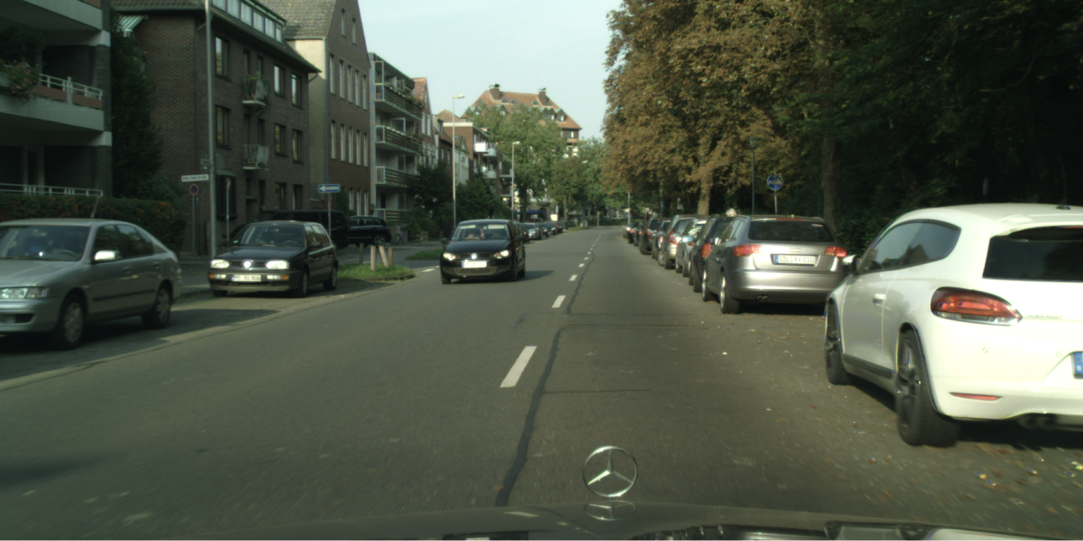
Figure 4a. Original image.
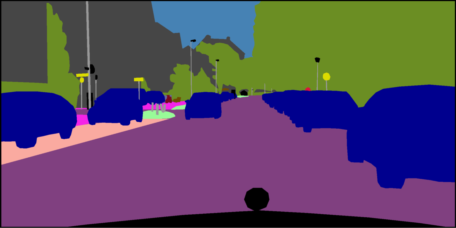
Figure 4b. Ground truth label.

Figure 4c. Output of TensorRT.
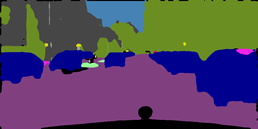
Figure 4d. Output of Keras.
Try it on other networks
Now you can try the ONNX workflow on other networks. For more information about good examples of segmentation networks, see Segmentation models with pretrained backbones on GitHub.
As an example, we show how to use the ONNX workflow with other networks. The network in this example is U-Net from the segmentation_models library. Here, we only loaded the model and did not train it. You may need to train these models on your preferred dataset.
One important point about these networks is that when you load these networks, their input layer sizes are as follows: (None, None, None, 3). To create a TensorRT engine, you need an ONNX file with a known input size. Before you convert this model to ONNX, change the network by assigning the size to its input and then convert it to the ONNX format.
As an example, load the U-Net network from this library (segmentation_models) and assign the size (244, 244, 3) to its input. After creating the TensorRT engine for the inference, do a similar conversion to what you did for semantic segmentation. Depending on the application and dataset, you may need to have a different color mapping.
 import segmentation_models as sm
 import keras
 from keras2onnx import convert_keras
 from engine import *

 onnx_path = 'unet.onnx'
 engine_name = 'unet.plan'
 batch_size = 1
 CHANNEL = 3
 HEIGHT = 224
 WIDTH = 224

 model = sm.Unet()
 model._layers[0].batch_input_shape = (None, 224,224,3)
 model = keras.models.clone_model(model)

 onx = convert_keras(model, onnx_path)
 with open(onnx_path, "wb") as f:
    f.write(onx.SerializeToString())


 shape = [batch_size , HEIGHT, WIDTH, CHANNEL]
 engine = build_engine(onnx_path, shape= shape)
 save_engine(engine, engine_name)
As we mentioned earlier in this post, another way of downloading pretrained models is to download them from NVIDIA NGC Models. It has a list of checkpoints for pretrained models. As an example you can search for UNet for TensorFlow and then go to the Download page to get the latest checkpoint.
Conclusion
In this post, we explained how to deploy deep learning applications using a TensorFlow-to-ONNX-to-TensorRT workflow, with several examples. The first example was ONNX-TensorRT on ResNet-50, and the second example was VGG16-based semantic segmentation that was trained on the Cityscapes Dataset. At the end of the post, we demonstrated how to apply this workflow on other networks. For more information about the best performance of training and inference, see NVIDIA Data Center Deep Learning Product Performance.
Houman Abbasian
Senior Deep Learning Software Engineer, NVIDIA
Yu-Te Cheng
Senior Deep Learning Engineer, Autonomous Driving Group, NVIDIA
Josh Park
Automotive Solutions Architect Manager, NVIDIA